\(\renewcommand\AA{\unicode{x212B}}\)

MonteCarloAbsorption v1

Summary

Calculates attenuation due to absorption and scattering in a sample & its environment using a Monte Carlo.

See Also

MayersSampleCorrection, CarpenterSampleCorrection, PearlMCAbsorption, VesuvioCalculateMS

Properties

Name	Direction	Type	Default	Description
InputWorkspace	Input	MatrixWorkspace	Mandatory	The name of the input workspace. The input workspace must have X units of wavelength.
OutputWorkspace	Output	MatrixWorkspace	Mandatory	The name to use for the output workspace.
NumberOfWavelengthPoints	Input	number	Optional	The number of wavelength points for which a simulation is attempted if ResimulateTracksForDifferentWavelengths=true
EventsPerPoint	Input	number	1000	The number of “neutron” events to generate per simulated point
SeedValue	Input	number	123456789	Seed the random number generator with this value
Interpolation	Input	string	Linear	Method of interpolation used to compute unsimulated values. Allowed values: [‘Linear’, ‘CSpline’]
SparseInstrument	Input	boolean	False	Enable simulation on special instrument with a sparse grid of detectors interpolating the results to the real instrument.
NumberOfDetectorRows	Input	number	5	Number of detector rows in the detector grid of the sparse instrument.
NumberOfDetectorColumns	Input	number	10	Number of detector columns in the detector grid of the sparse instrument.
MaxScatterPtAttempts	Input	number	5000	Maximum number of tries made to generate a scattering point within the sample (+ optional container etc). Objects with holes in them, e.g. a thin annulus can cause problems if this number is too low. If a scattering point cannot be generated by increasing this value then there is most likely a problem with the sample geometry.
ResimulateTracksForDifferentWavelengths	Input	boolean	False	Resimulate tracks for each wavelength point.
SimulateScatteringPointIn	Input	string	SampleAndEnvironment	Simulate the scattering point in the vicinity of the sample or its environment or both (default). Allowed values: [‘SampleAndEnvironment’, ‘SampleOnly’, ‘EnvironmentOnly’]

Description

This algorithm performs a Monte Carlo simulation to calculate the correction factors due to attenuation & single scattering within a sample plus optionally its sample environment.

Input Workspace Requirements

The algorithm will compute the correction factors on a bin-by-bin basis for each spectrum within the input workspace. The following assumptions on the input workspace will are made:

• X units are in wavelength

• the instrument is fully defined

• properties of the sample and optionally its environment have been set with SetSample

By default the beam is assumed to be the a slit with width and height matching the width and height of the sample. This can be overridden using SetBeam.

Method

By default, the material for the sample & containers will define the values of the cross section used to compute the absorption factor and will include contributions from both the total scattering cross section & absorption cross section. This follows the Hamilton-Darwin [1], [2] approach as described by T. M. Sabine in the International Tables of Crystallography Vol. C [3].

The algorithm proceeds as follows. For each spectrum:

1. find the associated detector position

2. find the associated efixed value (if applicable) & convert to wavelength (\(\lambda_{fixed}\))

3. for each event in NEvents

   • loop over the bins.

     • If ResimulateTracksForDifferentWavelengths = True then generate tracks using the following procedure for each wavelength step, where the size of each wavelength step is defined by NumberOfWavelengthPoints. If ResimulateTracksForDifferentWavelengths = false generate one set of tracks and define a step size of 1 ie all bins are visited. At the moment there are no wavelength dependent effects in the simulation that affect the simulation of the track geometry so the default value for ResimulateTracksForDifferentWavelengths is false. For each step (\(\lambda_{step}\))

     • generate a random point on the beam face defined by the input height & width. If the point is outside of the area defined by the face of the sample then it is pulled to the boundary of this area

     • generate a random point within the sample or container objects as the scatter point and create a Track from the selected position on the beam face to the scatter point

     • test for intersections of the track & sample/container objects, giving the number of subsections and corresponding distances within the object for each section, call them \(l_{1i}\)

     • form a second Track with the scatter position as the starting point and the direction defined by detPos - scatterPos

     • test for intersections of the track & sample/container objects, giving the number of subsections and corresponding distances within the object for each section, call them \(l_{2i}\)

     • define \(\lambda_1\) as the wavelength before scattering & \(\lambda_2\) as wavelength after scattering:

       • Direct: \(\lambda_1 = \lambda_1\), \(\lambda_2 = \lambda_{step}\)

       • Indirect: \(\lambda_1 = \lambda_{step}\), \(\lambda_2 = \lambda_{fixed}\)

       • Elastic: \(\lambda_1 = \lambda_2 = \lambda_{step}\)

     • compute the self-attenuation factor for all intersections as \(\prod\limits_{i} \exp(-(\rho_{1i}\sigma_{1i}(\lambda_{1i})l_{1i} + \rho_{2i}\sigma_{2i}(\lambda_{2i})l_{2i}))\) where \(\rho\) is the mass density of the material & \(\sigma\) the absorption cross-section at a given wavelength

     • accumulate this wavelength-specific factor across all NEvents

4. average the accumulated attentuation factors over NEvents and assign this as the correction factor for this \(\lambda_{step}\). Calculate the error as the standard deviation of the accumulated attenuation factors divided by \(\sqrt{NEvents}\)

5. finally, if ResimulateTracksForDifferentWavelengths = True, interpolate through the unsimulated wavelength points using the selected method

The algorithm generates some statistics on the number of scatter points generated in the sample and each environment component if the logging level is set to debug.

Interpolation

The default linear interpolation method will produce an absorption curve that is not smooth. CSpline interpolation will produce a smoother result by using a 3rd-order polynomial to approximate the original points - although if the data includes sudden changes it may introduce oscillations including negative values at the interpolated points.

The errors that the Monte Carlo simulation calculates for different wavelength points in a single spectrum may or may not be independent. If the same set of tracks have been used for different wavelengths (ResimulateTracksForDifferentWavelengths=False) then the errors will be correlated. A worst case positive correlation has been assumed giving an error on the interpolated point that is approximately the same as the surrounding simulated points.

If ResimulateTracksForDifferentWavelengths=True then the errors on the simulated points will be independent and the errors can be combined using standard formulae for combining errors on independent variables.

The error propagation through the spline interpolation is complex because each cubic polynomial is usually expressed as a function of the known y values and a derivative of those y values at the same points (some texts use the first derivative others the second). The error in y and the derivative of y are correlated at a particular x value and the derivatives at different x values are also correlated. So some extra covariances are required in addition to the error (variance) of each y value. The method followed [4] involves inverting a symmetric tridiagonal matrix and an analytic calculation for the inversion has been implemented to minimize the run time [6]

Sparse instrument

The simulation may take long to complete on instruments with a large number of detectors. To speed up the simulation, the instrument can be approximated by a sparse grid of detectors. The behavior can be enabled by setting the SparseInstrument property to true.

The sparse instrument consists of a grid of detectors covering the full instrument entirely. The figure below shows an example of a such an instrument approximating the IN5 spectrometer at ILL.

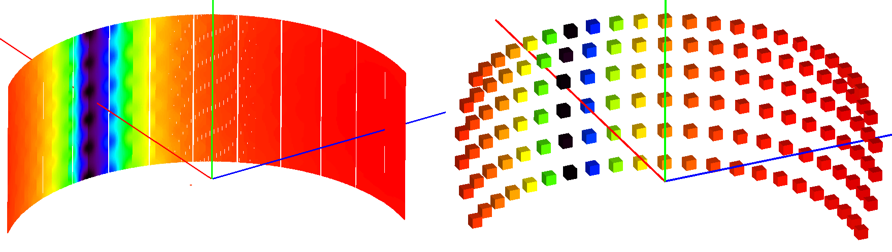
Absorption corrections for IN5 spectrometer interpolated from the sparse instrument shown on the right. The sparse instrument has 6 detector rows and 22 columns, a total of 132 detectors. IN5, on the other hand, has approximately 100000 detectors.

Note

It is recommended to remove monitor spectra from the input workspace since these are included in the area covered by the sparse instrument and may make the detector grid unnecessarily large.

When the sparse instrument option is enabled, a sparse instrument corresponding to the instrument attached to the input workspace is created. The simulation is then run using the created instrument. Finally, the simulated absorption corrections are interpolated to the output workspace.

The interpolation is a two step process: first a spatial interpolation is done from the detector grid of the sparse instrument to the actual detector positions of the full instrument. Then, if ResimulateTracksForDifferentWavelengths = True the correction factors are interpolated over the missing wavelengths.

Note

Currently, the sparse instrument mode does not support instruments with varying EFixed.

Spatial interpolation

The sample to detector distance does not matter for absorption, so it suffices to consider directions only. The detector grid of the sparse instrument consists of detectors at constant latitude and longitude intervals. For a detector \(D\) of the full input instrument at latitude \(\phi\) and longitude \(\lambda\), we pick the four detectors \(D_{ij}\) (\(i = 1, 2\) \(j = 1, 2\)) at the corners of the grid cell which includes (\(\phi\), \(\lambda\)).

If \(D\) coincides with any \(D_{ij}\), the \(y\) values of the histogram linked to \(D\) are directly taken from \(D_{ij}\). Otherwise, \(y\) is interpolated using a bilinear interpolation method. The data is interpolated in the longitude direction first:

\[ \begin{align}\begin{aligned}y_1 = \frac{(\lambda_2 - \lambda) * y_{11} + (\lambda - \lambda_1) * y_{21}}{\lambda_2 - \lambda_1}\\y_2 = \frac{(\lambda_2 - \lambda) * y_{12} + (\lambda - \lambda_1) * y_{22}}{\lambda_2 - \lambda_1},\end{aligned}\end{align} \]

and then finally in the latitude direction:

\[y = \frac{(\phi_2 - \phi) * y_1 + (\phi - \phi_1) * y_2}{\phi_2 - \phi_1}\]

The errors present in the 4 simulated histograms are assumed to be independent and they are propagated through the bilinear formulae given above to give one contribution to the error on the interpolated histogram. The second contribution is the interpolation error (how well the bilinear interpolation matches the actual attenuation factor variation). This is calculated based on the second derivative of the attenuation factor in the \(\phi\) and \(\lambda\) directions ([5])

Wavelength interpolation for sparse instruments

The wavelength points for simulation with the sparse instrument are chosen as follows:

1. Find the global minimum and maximum wavelengths of the input workspace.

2. Divide the wavelength interval to as many points as defined by the input parameters.

After the simulation has been run and the spatial interpolation done, the interpolated histograms will be further interpolated to the wavelength points of the input workspace. This is done similarly to the full instrument case. If only a single wavelength point is specified, then the output histograms will be filled with the single simulated value.

Note

If the input workspace contains varying bin widths then the output is always interpolated.

Usage

Example: A cylindrical sample with no container

data = CreateSampleWorkspace(WorkspaceType='Histogram', NumBanks=1)
data = ConvertUnits(data, Target="Wavelength")
# Default up axis is Y
SetSample(data, Geometry={'Shape': 'Cylinder', 'Height': 5.0, 'Radius': 1.0,
                  'Center': [0.0,0.0,0.0]},
                Material={'ChemicalFormula': '(Li7)2-C-H4-N-Cl6', 'SampleNumberDensity': 0.07})
# Simulating every data point can be slow. Use a smaller set and interpolate
abscor = MonteCarloAbsorption(data)
corrected = data/abscor

Example: A cylindrical sample with no container, resimulating tracks for different wavelengths, interpolating with a CSpline

data = CreateSampleWorkspace(WorkspaceType='Histogram', NumBanks=1)
data = ConvertUnits(data, Target="Wavelength")
# Default up axis is Y
SetSample(data, Geometry={'Shape': 'Cylinder', 'Height': 5.0, 'Radius': 1.0,
                  'Center': [0.0,0.0,0.0]},
                Material={'ChemicalFormula': '(Li7)2-C-H4-N-Cl6', 'SampleNumberDensity': 0.07})
# Simulating every data point can be slow. Use a smaller set and interpolate
abscor = MonteCarloAbsorption(data, ResimulateTracksForDifferentWavelengths=True, NumberOfWavelengthPoints=50,
                              Interpolation='CSpline')
corrected = data/abscor

Example: A cylindrical sample setting a beam size

data = CreateSampleWorkspace(WorkspaceType='Histogram', NumBanks=1)
data = ConvertUnits(data, Target="Wavelength")
# Default up axis is Y
SetSample(data, Geometry={'Shape': 'Cylinder', 'Height': 5.0, 'Radius': 1.0,
                  'Center': [0.0,0.0,0.0]},
                  Material={'ChemicalFormula': '(Li7)2-C-H4-N-Cl6', 'SampleNumberDensity': 0.07})
SetBeam(data, Geometry={'Shape': 'Slit', 'Width': 0.8, 'Height': 1.0})
# Simulating every data point can be slow. Use a smaller set and interpolate
abscor = MonteCarloAbsorption(data, NumberOfWavelengthPoints=50)
corrected = data/abscor

Example: A cylindrical sample with predefined container

The following example uses a test sample environment defined for the TEST_LIVE facility and ISIS_Histogram instrument and assumes that these are set as the default facility and instrument respectively. The definition can be found at [INSTALLDIR]/instrument/sampleenvironments/TEST_LIVE/ISIS_Histogram/CRYO-01.xml.

data = CreateSampleWorkspace(WorkspaceType='Histogram', NumBanks=1)
data = ConvertUnits(data, Target="Wavelength")
# Sample geometry is defined by container but not completely filled so
# we just define the height
SetSample(data, Environment={'Name': 'CRYO-01', 'Container': '8mm'},
          Geometry={'Height': 4.0},
          Material={'ChemicalFormula': '(Li7)2-C-H4-N-Cl6', 'SampleNumberDensity': 0.07})
# Simulating every data point can be slow. Use a smaller set and interpolate
abscor = MonteCarloAbsorption(data)
corrected = data/abscor

Example: A cylindrical sample using a sparse instrument description, interpolating with a CSpline

data = CreateSampleWorkspace(WorkspaceType='Histogram', NumBanks=1)
data = ConvertUnits(data, Target='Wavelength')
SetSample(data, Geometry={'Shape': 'Cylinder', 'Height': 5.0, 'Radius': 1.0,
                  'Center': [0.0,0.0,0.0]},
                Material={'ChemicalFormula': '(Li7)2-C-H4-N-Cl6', 'SampleNumberDensity': 0.07},
         )

abscor = MonteCarloAbsorption(data, SparseInstrument=True,
                              NumberOfDetectorRows=5, NumberOfDetectorColumns=5,
                              Interpolation='CSpline')
corrected = data/abscor

References

[1]

Darwin, C. G., Philos. Mag., 43 800 (1922) doi: 10.1080/10448639208218770

[2]

Hamilton, W.C., Acta Cryst, 10, 629 (1957) doi: 10.1107/S0365110X57002212

[3]

Sabine, T. M., International Tables for Crystallography, Vol. C, Page 609, Ed. Wilson, A. J. C and Prince, E. Kluwer Publishers (2004) doi: 10.1107/97809553602060000103

[4]

Gardner, James L., Journal of Research of the National Institute of Standards and Technology, section 4 (2003), https://nvlpubs.nist.gov/nistpubs/jres/108/1/j80gar.pdf

[5]

Severens, Ivo, technische universiteit eindhoven, (2003), https://www.win.tue.nl/casa/meetings/seminar/previous/_abstract030122_files/4.pdf

[6]

Hu, G. Y., O’Connell, R.F. , Journal of Physics A, 29 1511 (1996), doi: 10.1088/0305-4470/29/7/020 Note: the following edits have been applied to the formulae in the paper for the case -2 < D < 2: a) D = -2 cos \(\lambda\) has been implemented instead of D = 2 cos \(\lambda\) b) equation (10) has been modified for the -2 < D < 2 case so that the leading minus sign on the right hand side is removed

Categories: AlgorithmIndex | CorrectionFunctions\AbsorptionCorrections

Source

C++ header: MonteCarloAbsorption.h

C++ source: MonteCarloAbsorption.cpp