\(\renewcommand\AA{\unicode{x212B}}\)
Geometry of Shape
What is it?
In Mantid we use constructive solid geometry (CSG) to describe the shape of an object. This involves the creation of more complex shapes by the union, complement or intersection of simple primitive surfaces.
Why did we use CSG
Defining our object shape using CSG was selected for a number of reasons:
Using Surfaces based on mathematical equations rather than meshes of vertices give much better accuracy when tracking the interaction of particles through objects.
Scientists think in the shape of objects this way, for example if they have a sample that is a sphere radius 0.03m with a conical extrusion on top then that is exactly how they describe it in CSG. Otherwise they would need to be able to describe the co-ordinates for each vertex of the surface.
What shapes can be constructed
Mantid has direct support for creating various shapes directly, including
Sphere
Infinite Cylinder
Cylinder (finite height)
Slice of cylinder ring
Infinite Plane
Cuboid
Infinite Cone
Some of these shapes are infinite surfaces (the infinite plane, cone and cylinder) these are therefore not very useful on there own, but in combination with other shapes they can be capped as required.
For example if you cap and infinite Cylinder with two infinite planes you get a finite capped cylinder. This is in fact how the Cylinder shape is defined internally within Mantid.
For more on this see HowToDefineGeometricShape.
Calculating intersections between shapes
Intersection of a line and a cylinder
The line in Mantid is the equivalent of a ray in Math, and the cylinder here is referring to a cylindrical surface. The current intersection solver implemented in Mantid is using the parametrization method where a quadratic equation is solved to find the intersection point. This section will provide an in-depth derivation on how the final parameterization is formed, which is directly used in the source code.
For an arbitrary cylindrical surface, it can be uniquely defined by its radius \(r\) and symmetry axis \(\mathbf\epsilon\). Similarly, a line/ray can be uniquely defined by its starting point \(\mathbf{p}\) and direction vector (unit vector) \(\mathbf{\mu}\). Through parameterization, we can express an arbitrary line/ray in 3D as:
where \(\lambda\) is the distance one need to walk from the starting point along the direction of \(\mathbf{\mu}\) to reach a point on the line.
The parameterization of a random cylindrical surface in 3D can be complicated, but there is a simple mathematical expression when some special reference frame is used. More specifically, when the symmetry axis is one of the axis of the reference frame (using z-axis as an example here), a cylindrical surface can be expressed as:
The easiest way to solve for the intersection point is to plug the line parameterization into the equation above. However, this is not possible at the moment because the two equations are not in the same reference frame. Therefore, we need to convert the line parameterization parameters into the special cylindrical surface reference framework before we can solve for \(\lambda\).
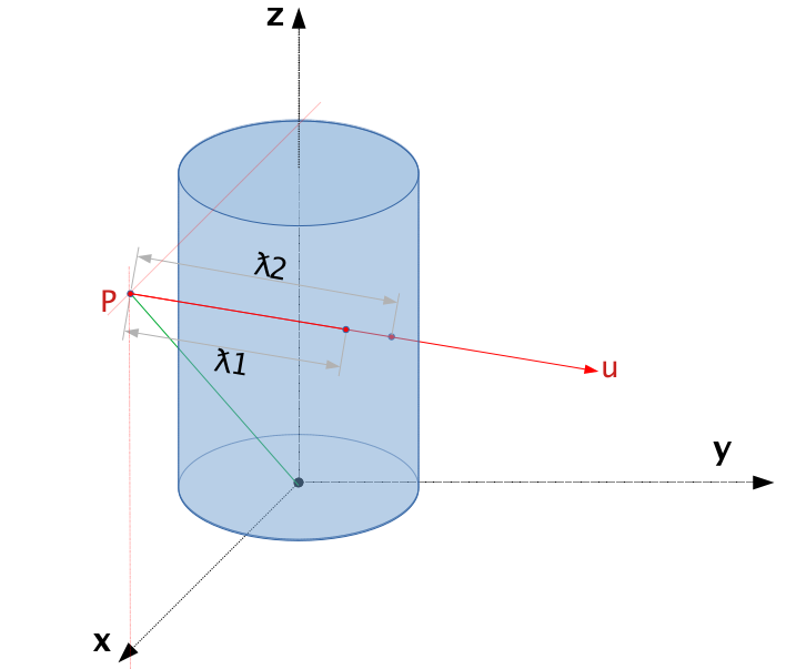
The figure above shows one of the special reference frame that can make the math a lot easier to handle. In this reference frame, the origin is a random point along the symmetry axis of the cylinder surface, and the symmetry axis is the z-axis. The starting point of the line, \(\mathbf{p}\) and the z-axis defines the x-z plane. In this reference frame, the expression for the cylindrical surface is exactly the same as the one shown above, and the line parameterization can be expressed as
Notice that \((p_x, p_y, p_z)\) are the covariance of \(\mathbf{p}\) in this special reference frame, and \((\mu_x, \mu_y, \mu_z)\) are the covariance of the direction vector \(\mathbf{\mu}\) in this reference frame. The remaining task is to find the value of \((p_x, p_y, p_z)\) and \((\mu_x, \mu_y, \mu_z)\) from \((p_0, p_1, p_2)\) and \((\mu_0, \mu_1, \mu_2)\).
Since \(\mathbf{p}\) is in the x-z plane, we get \(p_y = 0\) for free. Therefore, the remaining two covariance can be expressed as:
Notice that all the values on the left-hand are all in the special reference frame whereas the values on the right-hand are in the general/global reference frame.
Another thing worth mentioning here is that the expression above is assuming the special reference frame and the original reference frame share the same origin, which is true in most cases in mantid. However, if they are not the same, we need to take into consideration of the rigid-body shift due to change of origin, which can be easily done by:
where \(o_i\) is the covariance of the new origin in the general reference frame.
As for the covariances of the direction vector, the z component is relatively easy,
Finding the x component takes a little bit extra efforts. The x-axis of the special reference frame can be expressed as a unit vector:
Therefore,
Since direction vector is a unit vector, we can easily find
Now we can plug the line parameterization into the cylindrical surface equation to get the interception by solving for \(\lambda\), which gives us
For a standard quadratic equation, \(a_2x^2 + a_1x^1 + a_0x^0 = 0\), we have
and
and
Category: Concepts