IntegratePeaksProfileFitting v1¶

IntegratePeaksProfileFitting dialog.

Table of Contents

Summary
Properties
Description
- Similar algorithms
- Inputs
Calculations
Usage
Source

Summary ¶

Fits a series of peaks using 3D profile fitting as an Ikeda-Carpenter function by a bivariate gaussian.

Properties ¶

Name	Direction	Type	Default	Description
OutputPeaksWorkspace	Output	Workspace	Mandatory	PeaksWorkspace with integrated peaks
OutputParamsWorkspace	Output	Workspace	Mandatory	MatrixWorkspace with fit parameters
InputWorkspace	Input	Workspace	Mandatory	An input Sample MDHistoWorkspace or MDEventWorkspace in HKL.
PeaksWorkspace	Input	Workspace	Mandatory	PeaksWorkspace with peaks to be integrated.
RunNumber	Input	number	0	Run Number to integrate
DQPixel	Input	number	0.003	The side length of each voxel in the non-MD histogram used for fitting (1/Angstrom)
UBFile	Input	string		File containing the UB Matrix in ISAW format. Allowed extensions: [‘.mat’]
ModeratorCoefficientsFile	Input	string		File containing the Pade coefficients describing moderator emission versus energy. Allowed extensions: [‘.dat’]
StrongPeakParamsFile	Input	string		File containing strong peaks profiles. If left blank, no profiles will be enforced. Allowed extensions: [‘.pkl’]
IntensityCutoff	Input	number	0	Minimum number of counts to force a profile
EdgeCutoff	Input	number	0	Pixels within EdgeCutoff from a detector edge will be have a profile forced. Currently for 256x256 cameras only.
FracHKL	Input	number	0.5	Fraction of HKL to consider for profile fitting.
FracStop	Input	number	0.05	Fraction of max counts to include in peak selection.
MinpplFrac	Input	number	0.9	Min fraction of predicted background level to check
MaxpplFrac	Input	number	1.1	Max fraction of predicted background level to check
MindtBinWidth	Input	number	15	Smallest spacing (in microseconds) between data points for TOF profile fitting.
NTheta	Input	number	50	Number of bins for bivarite Gaussian along the scattering angle.
NPhi	Input	number	50	Number of bins for bivariate Gaussian along the azimuthal angle.
DQMax	Input	number	0.15	Largest total side length (in Angstrom) to consider for profile fitting.
DtSpread	Input	number	0.03	The fraction of the peak TOF to consider for TOF profile fitting.
PeakNumber	Input	number	-1	Which Peak to fit. Leave negative for all.

This algorithm performs integration of single crystal Bragg peaks by fitting the intensity distribution as a 3D distribution made of an Ikeda-Carpenter function (TOF coordinate) and a bivariate Normal distribution.

Similar algorithms ¶

See IntegratePeaksMD v2 or IntegrateEllipsoids v1 for peak-minus-background integration algorithms in reciprocal space.

Inputs ¶

The algorithms takes two input workspaces:

A MDEventWorkspace containing the events in multi-dimensional space. This would be the output of ConvertToMD v1.
As well as a PeaksWorkspace containing single-crystal peak locations. This could be the output of FindPeaksMD v1 or PredictPeaks v1
The OutputPeaksWorkspace will contain a copy of the input PeaksWorkspace, with the integrated intensities and errors changed.
The OutputParamsWorkspace is a TableWorkspace containing the fit parameters. Peaks which could not be fit are omitted.

Calculations ¶

This algorithm will fit a set of peaks in a PeaksWorkspace. The intensity profile is fit to an MDHisto workspace formed around the peak location.

Constructing the Measured Intensity Distribution ¶

To construct the measured distribution to be fit, a histogram of events is made around the peak. This histogram is in (q_x, q_y, q_z) and composed of voxels of side length dQPixel. To minimize the effect of neighboring peaks on profile fitting, the variable qMask is used to only consider a region around the peak in (h,k,l) space. It will filter voxels outside of (h ± fracHKL, k ± fracHKL, l ± fracHKL) from calculations used for profile fitting. In practice, values of 0.35 < fracHKL < 0.5 seem to work best.

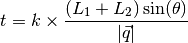
Fitting the Time-of-Flight Coordinate ¶

The time-of-flight (TOF), t, of each voxel is determined as:

$t = k \times \frac{(L_1 + L_2)\sin(\theta)}{|\vec{q}|}$

The events are histogrammed by their t values to create a TOF profile. This profile can then be fit to the Ikeda Carpenter function. To separate the peak and background, different levels of intensity are filtered out. The predicted background level is determined as the average background not near the peak or off the edge and values within minppl_frac and maxppl_frac times the predicted value are tried. The best fit to the expected moderator emission (determined by the moderator coefficients defined in ModeratorCoefficientsFile) is taken and these voxels are considered to be signal.

Fitting the Non-TOF Coordinate ¶

TOF goes as $1/|\vec{q}|$ and so it is natural to use spherical coordinate. In that sense, the other two coordinates are $(q_{\theta} , q_{\phi_az})$ - along the scattering angle and azimuthal angle, respectively. From the MDHisto Workspace (filtered by qMask and using only the signal voxels from the TOF fight), a 2D histogram is constructed which is fit to a bivariate normal distribution. The histogram has nTheta $\times$ nPhi bins.

For weak peaks or peaks near detector edges, the 2D histogram likely does not reflect the full profile. To address this, the profile of the nearest strong peaks is forced when doing the BVG fit. The profile is fit (allowed to vary 10% in $\sigma_x, \sigma_y, \rho$ ) and location and amplitude are not fixed. Weak peaks are defined as peaks with fewer than forceCutoff counts from peak-minus-background integration or within dEdge pixels of the detector edge.

Integrating the Model ¶

The final intensity profile is given by

$Y(\vec{q}) = A \times Y_{TOF}(\vec{q}) \times Y_{BVG}(\vec{q}) + B$

where $A$ and $B$ are scaling constants. Here the background is assumed to be constant $B$ over the volume of the peak, so the model of the peak itself is $Y_{model}(\vec{q}) = A \times Y_{TOF}(\vec{q}) \times Y_{BVG}(\vec{q})$ . The peak intensity $I$ , is given by summing $Y_{model}(\vec{q})$ over voxels which are greater than FracStop of the maximum.

$\sigma(I)$ is given as

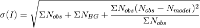
$\sigma(I) = \sqrt{\Sigma N_{obs} + \Sigma N_{BG} + \frac{\Sigma N_{obs}(N_{obs}-N_{model})^2}{\Sigma N_{obs}}}$

where the first two terms come from Poissionian statistics and the final term is the variance of the fit. Those sums are over the same voxels used to calculate intensity.

Usage ¶

Example - IntegratePeaksProfileFitting

 Load(Filename='/SNS/MANDI/IPTS-8776/0/5921/NeXus/MANDI_5921_event.nxs', OutputWorkspace='MANDI_5921_event')
 MANDI_5921_md = ConvertToMD(InputWorkspace='MANDI_5921_event',  QDimensions='Q3D', dEAnalysisMode='Elastic',
                          Q3DFrames='Q_lab', QConversionScales='Q in A^-1',
                          MinValues='-5, -5, -5', Maxvalues='5, 5, 5', MaxRecursionDepth=10,
                          LorentzCorrection=False)
 LoadIsawPeaks(Filename='/SNS/MANDI/shared/ProfileFitting/demo_5921.integrate', OutputWorkspace='peaks_ws')

 IntegratePeaksProfileFitting(OutputPeaksWorkspace='peaks_ws_out', OutputParamsWorkspace='params_ws',
         InputWorkspace='MANDI_5921_md', PeaksWorkspace='peaks_ws', RunNumber=5921, DtSpread=0.015,
         UBFile='/SNS/MANDI/shared/ProfileFitting/demo_5921.mat',
         ModeratorCoefficientsFile='/SNS/MANDI/shared/ProfileFitting/franz_coefficients_2017.dat',
         MinpplFrac=0.9, MaxpplFrac=1.1, MindtBinWidth=15,
         StrongPeakParamsFile='/SNS/MANDI/shared/ProfileFitting/strongPeakParams_beta_lac_mut_mbvg.pkl',
         peakNumber=30)

Categories: Algorithms | Crystal\Integration

Source ¶

Python: IntegratePeaksProfileFitting.py (last modified: 2018-06-22)