MonteCarloAbsorption v1¶

MonteCarloAbsorption dialog.

Table of Contents

Summary
- See Also
Properties
Description
Usage
References
Source

Summary ¶

Calculates attenuation due to absorption and scattering in a sample & its environment using a Monte Carlo.

Properties ¶

Name	Direction	Type	Default	Description
InputWorkspace	Input	MatrixWorkspace	Mandatory	The name of the input workspace. The input workspace must have X units of wavelength.
OutputWorkspace	Output	MatrixWorkspace	Mandatory	The name to use for the output workspace.
NumberOfWavelengthPoints	Input	number	Optional	The number of wavelength points for which a simulation is attempted (default: all points)
EventsPerPoint	Input	number	300	The number of “neutron” events to generate per simulated point
SeedValue	Input	number	123456789	Seed the random number generator with this value
Interpolation	Input	string	Linear	Method of interpolation used to compute unsimulated values. Allowed values: [‘Linear’, ‘CSpline’]
SparseInstrument	Input	boolean	False	Enable simulation on special instrument with a sparse grid of detectors interpolating the results to the real instrument.
NumberOfDetectorRows	Input	number	5	Number of detector rows in the detector grid of the sparse instrument.
NumberOfDetectorColumns	Input	number	10	Number of detector columns in the detector grid of the sparse instrument.
MaxScatterPtAttempts	Input	number	5000	Maximum number of tries made to generate a scattering point within the sample (+ optional container etc). Objects with holes in them, e.g. a thin annulus can cause problems if this number is too low. If a scattering point cannot be generated by increasing this value then there is most likely a problem with the sample geometry.

Description ¶

This algorithm performs a Monte Carlo simulation to calculate the correction factors due to attenuation & single scattering within a sample plus optionally its sample environment.

Input Workspace Requirements ¶

The algorithm will compute the correction factors on a bin-by-bin basis for each spectrum within the input workspace. The following assumptions on the input workspace will are made:

X units are in wavelength
the instrument is fully defined
properties of the sample and optionally its environment have been set with SetSample

By default the beam is assumed to be the a slit with width and height matching the width and height of the sample. This can be overridden using SetBeam.

By default, the material for the sample & containers will define the values of the cross section used to compute the absorption factor and will include contributions from both the total scattering cross section & absorption cross section. This follows the Hamilton-Darwin [1], [2] approach as described by T. M. Sabine in the International Tables of Crystallography Vol. C [3].

The algorithm proceeds as follows. For each spectrum:

find the associated detector position
find the associated efixed value (if applicable) & convert to wavelength ( $\lambda_{fixed}$ )
loop over the bins in steps defined by NumberOfWavelengthPoints and for each step ()
- define as the wavelength before scattering & as wavelength after scattering:
  - Direct: $\lambda_1 = \lambda_1$ , $\lambda_2 = \lambda_{step}$
  - Indirect: $\lambda_1 = \lambda_{step}$ , $\lambda_2 = \lambda_{fixed}$
  - Elastic: $\lambda_1 = \lambda_2 = \lambda_{step}$
- for each event in NEvents:
  - generate a random point on the beam face defined by the input height & width. If the point is outside of the area defined by the face of the sample then it is pulled to the boundary of this area
  - generate a random point within the sample or container objects as the scatter point and create a Track from the selected position on the beam face to the scatter point
  - test for intersections of the track & sample/container objects, giving the number of subsections and corresponding distances within the object for each section, call them $l_{1i}$
  - form a second Track with the scatter position as the starting point and the direction defined by detPos - scatterPos
  - test for intersections of the track & sample/container objects, giving the number of subsections and corresponding distances within the object for each section, call them $l_{2i}$
  - compute the self-attenuation factor for all intersections as $\prod\limits_{i} \exp(-(\rho_{1i}\sigma_{1i}(\lambda_{1i})l_{1i} + \rho_{2i}\sigma_{2i}(\lambda_{2i})l_{2i}))$ where $\rho$ is the mass density of the material & $\sigma$ the absorption cross-section at a given wavelength
  - accumulate this factor with the factor for all NEvents
- average the accumulated attentuation factors over NEvents and assign this as the correction factor for this $\lambda_{step}$ .
finally, interpolate through the unsimulated wavelength points using the selected method

Interpolation ¶

The default linear interpolation method will produce an absorption curve that is not smooth. CSpline interpolation will produce a smoother result by using a 3rd-order polynomial to approximate the original points.

Sparse instrument ¶

The simulation may take long to complete on instruments with a large number of detectors. To speed up the simulation, the instrument can be approximated by a sparse grid of detectors. The behavior can be enabled by setting the SparseInstrument property to true.

The sparse instrument consists of a grid of detectors covering the full instrument entirely. The figure below shows an example of a such an instrument approximating the IN5 spectrometer at ILL.

IN5 spectrometer and its sparse approximation.

Absorption corrections for IN5 spectrometer interpolated from the sparse instrument shown on the right. The sparse instrument has 6 detector rows and 22 columns, a total of 132 detectors. IN5, on the other hand, has approximately 100000 detectors.

Note

It is recommended to remove monitor spectra from the input workspace since these are included in the area covered by the sparse instrument and may make the detector grid unnecessarily large.

When the sparse instrument option is enabled, a sparse instrument corresponding to the instrument attached to the input workspace is created. The simulation is then run using the created instrument. Finally, the simulated absorption corrections are interpolated to the output workspace.

The interpolation is a two step process: first a spatial interpolation is done from the detector grid of the sparse instrument to the actual detector positions of the full instrument. Then, the correction factors are interpolated over the missing wavelengths.

Note

Currently, the sparse instrument mode does not support instruments with varying EFixed.

Spatial interpolation ¶

The sample to detector distance does not matter for absorption, so it suffices to consider directions only. The detector grid of the sparse instrument consists of detectors at constant latitude and longitude intervals. For a detector $D$ of the full input instrument at latitude $\phi$ and longitude $\lambda$ , we pick the four detectors $D_i$ ( $i = 1, 2, 3, 4$ ) at the corners of the grid cell which includes ( $\phi$ , $\lambda$ ). The distance $\Delta_i$ in units of angle between $D$ and $D_i$ on a spherical surface is given by

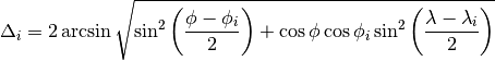
$\Delta_i = 2 \arcsin \sqrt{\sin^2 \left(\frac{\phi - \phi_i}{2} \right) + \cos \phi \cos \phi_i \sin^2 \left( \frac{\lambda - \lambda_i}{2} \right)}$

If $D$ coincides with any $D_i$ , the $y$ values of the histogram linked to $D$ are directly taken from $D_i$ . Otherwise, $y$ is interpolated using the inverse distance weighing method

$y = \frac{\sum_i w_i y_i}{\sum_i w_i},$

where the weights are given by

$w_i = \frac{1}{\Delta_i^2}$

Wavelength interpolation ¶

The wavelength points for simulation with the sparse instrument are chosen as follows:

Find the global minimum and maximum wavelengths of the input workspace.
Divide the wavelength interval to as many points as defined by the input parameters.

After the simulation has been run and the spatial interpolation done, the interpolated histograms will be further interpolated to the wavelength points of the input workspace. This is done similarly to the full instrument case. If only a single wavelength point is specified, then the output histograms will be filled with the single simulated value.

Note

If the input workspace contains varying bin widths then the output is always interpolated.

Usage ¶

Example: A cylindrical sample with no container

data = CreateSampleWorkspace(WorkspaceType='Histogram', NumBanks=1)
data = ConvertUnits(data, Target="Wavelength")
# Default up axis is Y
SetSample(data, Geometry={'Shape': 'Cylinder', 'Height': 5.0, 'Radius': 1.0,
                  'Center': [0.0,0.0,0.0]},
                Material={'ChemicalFormula': '(Li7)2-C-H4-N-Cl6', 'SampleNumberDensity': 0.07})
# Simulating every data point can be slow. Use a smaller set and interpolate
abscor = MonteCarloAbsorption(data, NumberOfWavelengthPoints=50)
corrected = data/abscor

Example: A cylindrical sample with no container, interpolating with a CSpline

data = CreateSampleWorkspace(WorkspaceType='Histogram', NumBanks=1)
data = ConvertUnits(data, Target="Wavelength")
# Default up axis is Y
SetSample(data, Geometry={'Shape': 'Cylinder', 'Height': 5.0, 'Radius': 1.0,
                  'Center': [0.0,0.0,0.0]},
                Material={'ChemicalFormula': '(Li7)2-C-H4-N-Cl6', 'SampleNumberDensity': 0.07})
# Simulating every data point can be slow. Use a smaller set and interpolate
abscor = MonteCarloAbsorption(data, NumberOfWavelengthPoints=50,
                              Interpolation='CSpline')
corrected = data/abscor

Example: A cylindrical sample setting a beam size

data = CreateSampleWorkspace(WorkspaceType='Histogram', NumBanks=1)
data = ConvertUnits(data, Target="Wavelength")
# Default up axis is Y
SetSample(data, Geometry={'Shape': 'Cylinder', 'Height': 5.0, 'Radius': 1.0,
                  'Center': [0.0,0.0,0.0]},
                  Material={'ChemicalFormula': '(Li7)2-C-H4-N-Cl6', 'SampleNumberDensity': 0.07})
SetBeam(data, Geometry={'Shape': 'Slit', 'Width': 0.8, 'Height': 1.0})
# Simulating every data point can be slow. Use a smaller set and interpolate
abscor = MonteCarloAbsorption(data, NumberOfWavelengthPoints=50)
corrected = data/abscor

Example: A cylindrical sample with predefined container

The following example uses a test sample environment defined for the TEST_LIVE facility and ISIS_Histogram instrument and assumes that these are set as the default facility and instrument respectively. The definition can be found at [INSTALLDIR]/instrument/sampleenvironments/TEST_LIVE/ISIS_Histogram/CRYO-01.xml.

data = CreateSampleWorkspace(WorkspaceType='Histogram', NumBanks=1)
data = ConvertUnits(data, Target="Wavelength")
# Sample geometry is defined by container but not completely filled so
# we just define the height
SetSample(data, Environment={'Name': 'CRYO-01', 'Container': '8mm'},
          Geometry={'Height': 4.0},
          Material={'ChemicalFormula': '(Li7)2-C-H4-N-Cl6', 'SampleNumberDensity': 0.07})
# Simulating every data point can be slow. Use a smaller set and interpolate
abscor = MonteCarloAbsorption(data, NumberOfWavelengthPoints=30)
corrected = data/abscor

Example: A cylindrical sample setting a beam size

data = CreateSampleWorkspace(WorkspaceType='Histogram', NumBanks=1)
data = ConvertUnits(data, Target='Wavelength')
SetSample(data, Geometry={'Shape': 'Cylinder', 'Height': 5.0, 'Radius': 1.0,
                  'Center': [0.0,0.0,0.0]},
                Material={'ChemicalFormula': '(Li7)2-C-H4-N-Cl6', 'SampleNumberDensity': 0.07},
         )

abscor = MonteCarloAbsorption(data, NumberOfWavelengthPoints=10,SparseInstrument=True,
                              NumberOfDetectorRows=5, NumberOfDetectorColumns=5)
corrected = data/abscor

References ¶

[1]	Darwin, C. G., Philos. Mag., 43 800 (1922) doi: 10.1080/10448639208218770

[2]	Hamilton, W.C., Acta Cryst, 10, 629 (1957) doi: 10.1107/S0365110X57002212

[3]	Sabine, T. M., International Tables for Crystallography, Vol. C, Page 609, Ed. Wilson, A. J. C and Prince, E. Kluwer Publishers (2004) doi: 10.1107/97809553602060000103

Categories: Algorithms | CorrectionFunctions\AbsorptionCorrections

Source ¶

C++ source: MonteCarloAbsorption.cpp (last modified: 2017-10-03)

C++ header: MonteCarloAbsorption.h (last modified: 2018-05-07)

MonteCarloAbsorption v1¶

Summary ¶

See Also ¶

Properties ¶

Description ¶

Input Workspace Requirements ¶

Method ¶

Interpolation ¶

Sparse instrument ¶

Spatial interpolation ¶

Wavelength interpolation ¶

Usage ¶

References ¶

Source ¶