Minimizers play a central role when Fitting a model in Mantid. Given the following elements:
The minimizer is the method that adjusts the function parameters so that the model fits the data as closely as possible. The cost function defines the concept of how close a fit is to the data. See the general concept page on Fitting for a broader discussion of how these components interplay when fitting a model with Mantid.
Several minimizers are included with Mantid and can be selected in the Fit Function property browser or when using the algorithm Fit The following options are available:
Levenberg-Marquardt (default)
Levenberg-MarquardtMD
A Levenberg-Marquardt implementation generalised to allow different cost functions, and supporting chunking techniques for large datasets.
Damping
A Gauss-Newton algorithm with damping.
All these algorithms are iterative. The Simplex algorithm, also known as Nelder–Mead method, belongs to the class of optimization algorithms without derivatives, or derivative-free optimization. Note that here simplex refers to downhill simplex optimization. Steepest descent and the two variants of Conjugate Gradient included with Mantid (Fletcher-Reeves and Polak-Ribiere) belong to the class of optimization or minimization algorithms generally known as conjugate gradient, which use first-order derivatives. The derivatives are calculated with respect to the cost function to drive the iterative process towards a local minimum.
BFGS and the Levenberg-Marquardt algorithms belong to the second-order class of algorithms, in the sense that they use second-order information of the cost function (second derivatives or the Hessian matrix). Some algorithms like BFGS approximate the Hessian by the gradient values of successive iterations. The Levenberg-Marquard algorithm is a modified Gauss-Newton that introduces an adaptive term to prevent unstability when the approximated Hessian is not positive defined. An in-depth description of the methods is beyond the scope of these pages. More information can be found from the links and general references on optimization methods such as [Kelley1999] and [NocedalAndWright2006].
Finally, FABADA is an algorithm for Bayesian data analysis. It is excluded from the comparison described below, as it is a substantially different algorithm.
In most cases, the implementation of these algorithms is based on the GNU Scientific Libraty routines for least-squares fitting
Here we describe a comparison of minimizers available in Mantid, in terms of how they perform when fitting several benchmark problems. This is a relative comparison in the sense that for every problem the best possible results with Mantid minimizers are given a top score of “1”. The ranking is continuous and the score of a minimizer represents the ratio between its performance and the performance of the best. We compare accuracy and run time.
For example, a ranking of 1.25 for a minimizer for a given problem means:
All the minimizers available in Mantid 3.7 were compared, with the exception of FABADA which belongs to a different class of methods and would not be compared in a fair manner. For all the minimizers compared here the algorithm Fit was run using the same initialization or starting points for test every problem, as specified in the test problem definitions. No constraints or ties were added.
Accuracy is measured using the sum of squared fitting errors as
metric, or “ChiSquared” as defined in Fit, where the fitting errors are the
difference between the expected outputs and the outputs calculated by
the model fitted: 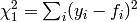 (see
CalculateChiSquared for full details
and different variants). Run time is measured for the execution of
the Fit algorithm for an equation and dataset
previously created.
(see
CalculateChiSquared for full details
and different variants). Run time is measured for the execution of
the Fit algorithm for an equation and dataset
previously created.
The cost function used in this general comparison is ‘Least squares’ but without using input error estimates (see details below).
Each test problem included in this comparison is defined by the following information:
 values)
 values)
The problems have been obtained from the following benchmark:
As the test problems do not define observational errors this comparison does not use the weights of the least squares cost function. An alternative comparison using simulated errors is also available, with similar results overall.
The summary table shows the median ranking across all the test problems. See detailed results by test problem (accuracy).
Alternatively, see the detailed results when using weighted least squares as cost function.
| BFGS | Conjugate gradient (Fletcher-Reeves imp.) | Conjugate gradient (Polak-Ribiere imp.) | Damping | Levenberg-Marquardt | Levenberg-MarquardtMD | Simplex | SteepestDescent | |
|---|---|---|---|---|---|---|---|---|
| NIST, “lower” difficulty | 3.841 | 3.003 | 3.003 | 1 | 1 | 1 | 1.017 | 6.436 |
| NIST, “average” difficulty | 269 | 22.35 | 22.5 | 1 | 1 | 1 | 79.31 | 315.9 |
| NIST, “higher” difficulty | 36.33 | 10.82 | 8.366 | 1.847 | 1 | 1 | 18.55 | 100.7 |
The summary table shows the median ranking across all the test problems. See detailed results by test problem (run time).
Alternatively, see the detailed results when using weighted least squares as cost function.
| BFGS | Conjugate gradient (Fletcher-Reeves imp.) | Conjugate gradient (Polak-Ribiere imp.) | Damping | Levenberg-Marquardt | Levenberg-MarquardtMD | Simplex | SteepestDescent | |
|---|---|---|---|---|---|---|---|---|
| NIST, “lower” difficulty | 1.258 | 1.412 | 1.391 | 1 | 1.094 | 1.036 | 1.622 | 11.83 |
| NIST, “average” difficulty | 1.326 | 9.579 | 7.935 | 1 | 1.11 | 1.035 | 1.901 | 12.97 |
| NIST, “higher” difficulty | 1.02 | 1.84 | 2.155 | 1.244 | 1.044 | 1.198 | 1.206 | 5.321 |
References:
| [Kelley1999] | Kelley C.T. (1999). Iterative Methods for Optimization. SIAM series in Applied Mathematics. Frontiers in Applied Mathematics, vol. 18. ISBN: 978-0-898714-33-3. |
| [NocedalAndWright2006] | Nocedal J, Wright S. (2006). Numerical Optimization, 2nd edition. pringer Series in Operations Research and Financial Engineering. DOI: 10.1007/978-0-387-40065-5 |
Category: Concepts