\(\renewcommand\AA{\unicode{x212B}}\)

ComputeIncoherentDOS v1

Summary

Calculates the neutron weighted generalised phonon density of states in the incoherent approximation from a measured powder INS MatrixWorkspace

Properties

Name	Direction	Type	Default	Description
InputWorkspace	Input	MatrixWorkspace	Mandatory	Input MatrixWorkspace containing the reduced inelastic neutron spectrum in (Q,E) or (2theta,E) space.
Temperature	Input	number	300	Sample temperature in Kelvin.
MeanSquareDisplacement	Input	number	0	Average mean square displacement in Angstrom^2.
QSumRange	Input	string	0,Qmax	Range in Q (in Angstroms^-1) to sum data over.
EnergyBinning	Input	string	0,Emax/50,Emax*0.9	Energy binning parameters [Emin, Emax] or [Emin, Estep, Emax] in meV.
Wavenumbers	Input	boolean	False	Should the output be in Wavenumbers (cm^-1)?
StatesPerEnergy	Input	boolean	False	Should the output be in states per unit energy rather than mb/sr/fu/energy? (Only for pure elements, need to set the sample material information)
OutputWorkspace	Output	MatrixWorkspace	Mandatory	Output workspace name.
TwoThetaSumRange	Input	string	Twothetamin, Twothetamax	Range in 2theta (in degrees) to sum data over.

Description

Computes the phonon density of states from an inelastic neutron scattering measurement of a powder or polycrystalline sample, assuming that all scattering is incoherent, using the formula for the 1-phonon incoherent scattering function [1]:

\[S^{(1)}_{\mathrm{inc}}(Q,E) = \exp\left(-2\bar{W}(Q)\right) \frac{Q^2}{E} \left< n+\frac{1}{2}\pm\frac{1}{2} \right> \left[ \sum_k \frac{\sigma_k^{\mathrm{scatt}}}{2m_k} g_k(E) \right],\]

where the term in square brackets is the neutron weighted density of states which is calculated by this algorithm, and \(g_k(E)\) is the partial density of states for each component (element or isotope) \(k\) in the material. \(m_k\) is the relative atomic mass of the component.

The average Debye-Waller factor \(\exp\left(-2\bar{W}(Q)\right)\) is calculated using an average mean-square displacement \(\langle u^2 \rangle\), using \(W=Q^2\langle u^2\rangle/2\).

\(\langle u^2 \rangle\) is also called the isotropic atomic displacement parameter \(U_{\mathrm{iso}}\) in Rietveld refinement programs like GSAS. There is also another, related, type of atomic displacement parameter used in programs like FullProf called \(B_{\mathrm{iso}}\) : \(B_{\mathrm{iso}}=8\pi^2U_{\mathrm{iso}}\) [2].

The algorithm accepts both \(S(Q,E)\) workspaces as well as \(S(2\theta,E)\) workspaces. In the latter case \(Q\) values are calculated from \(2\theta\) and \(E\) before applying the formula above. Note, that QSumRange is only applicable with \(S(Q,E)\) while TwoThetaSumRange works only for \(S(2\theta,E)\).

If the data has been normalised to a Vanadium standard measurement, the output of this algorithm is the neutron weighted density of states in milibarns/steradians per formula unit per meV (or per cm^-1). If the sample material has been set and is found to be a pure element, then an additional option will be enabled to calculate the DOS in states per meV (states per cm^-1) by dividing by the scattering cross-section and multiplying by the relative atomic mass.

Restrictions on the Input Workspace

The input workspace must have units of Momentum Transfer or Degrees and contain histogram data with common binning on all spectra.

Usage

Note

To run these usage examples please first download the usage data, and add these to your path. In Mantid this is done using Manage User Directories.

ISIS Example

The following code will run a reduction on a MARI (ISIS) dataset and apply the algorithm to the reduced data. The datafiles (runs 21334, 21335, 21347) and map file ‘mari_res2013.map’ should be in your path. Run number 21335 is a measurement of a large Aluminium sample from the neutron training course.

from Direct import DirectEnergyConversion
from mantid.simpleapi import *
rd = DirectEnergyConversion.DirectEnergyConversion('MARI')
ws = rd.convert_to_energy(21334, 21335, 60, [-55,0.05,55], 'mari_res2013.map',
    monovan_run=21347, sample_mass=106.4, sample_rmm=27, monovan_mapfile='mari_res2013.map')
ws_sqw = SofQW3(ws, [0,0.1,12], 'Direct', 60)
SetSampleMaterial(ws_sqw,'Al')
ws_dos = ComputeIncoherentDOS(ws_sqw, Temperature=5, StatesPerEnergy=True)

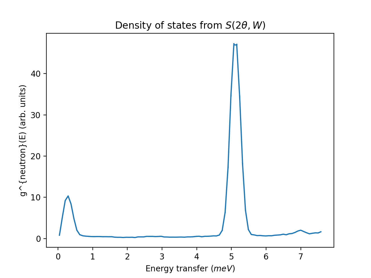
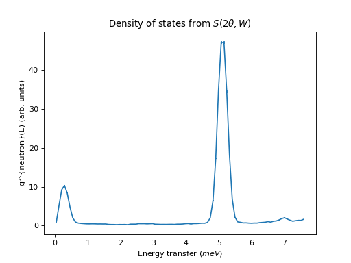
ILL Example using S(2theta, E) as input

from mantid import mtd
from mantid.simpleapi import *
import matplotlib.pyplot as plt

ws = DirectILLCollectData('ILL/IN4/087294.nxs')
DirectILLReduction(ws, OutputWorkspace='sqw', OutputSofThetaEnergyWorkspace='stw')
temperature = ws.run().getProperty('sample.temperature').value
dos = ComputeIncoherentDOS('stw',  Temperature=temperature, EnergyBinning='0, Emax')

fig, axis = plt.subplots(subplot_kw={'projection':'mantid'})
axis.errorbar(dos)
axis.set_title('Density of states from $S(2\\theta,W)$')
# Uncomment the line below to show the plot.
#fig.show()
mtd.clear()

(Source code, png, hires.png, pdf)

Test Example

This example uses a generated dataset so that it will run on automated tests of the build system where the above datafiles do not exist.

ws = CreateSampleWorkspace(binWidth = 0.1, XMin = 0, XMax = 50, XUnit = 'DeltaE')
ws = ScaleX(ws, -25, "Add")
LoadInstrument(ws, InstrumentName='MARI', RewriteSpectraMap = True)
ws = SofQW(ws, [0, 0.05, 8], 'Direct', 25)
ws_DOS = ComputeIncoherentDOS(ws)

References

[1]

Thermodynamic Properties of Solids, eds. Chaplot, Mittal, Choudhury, Chapter 3

[2]

GSAS Manual, page 123

Categories: AlgorithmIndex | Inelastic

Source

Python: ComputeIncoherentDOS.py