SassenaFFT v1#
Summary#
Performs complex Fast Fourier Transform of intermediate scattering function
See Also#
ExtractFFTSpectrum, FFT, FFTDerivative, MaxEnt, RealFFT, FFTSmooth
Properties#
Name |
Direction |
Type |
Default |
Description |
|---|---|---|---|---|
InputWorkspace |
InOut |
WorkspaceGroup |
Mandatory |
The name of the input group workspace |
FFTonlyRealPart |
Input |
boolean |
False |
Do we FFT only the real part of I(Q,t)? (optional, default is False) |
DetailedBalance |
Input |
boolean |
False |
Do we apply detailed balance condition? (optional, default is False) |
Temp |
Input |
number |
300 |
Multiply structure factor by exp(E/(2*kT) |
Description#
The Sassena application generates
intermediate scattering factors from molecular dynamics trajectories.
This algorithm reads Sassena output and stores all data in workspaces of
type Workspace2D, grouped under a single
WorkspaceGroup. It is implied that the time unit is
one picosecond.
Sassena output files are in HDF5 format, and can be made up of the following datasets: qvectors, fq, fq0, fq2, and fqt
The group workspace should contain workspaces _fqt.Re and _fqt.Im containing the real and imaginary parts of the intermediate structure factor, respectively. This algorithm will take both and perform FFT v1, storing the real part of the transform in workspace _fqw and placing this workspace under the input group workspace. Assuming the time unit to be one picosecond, the resulting energies will be in units of one micro-eV.
The Schofield correction (P. Schofield, Phys. Rev. Letters 4(5), 239 (1960)) is optionally applied to the resulting dynamic structure factor to reinstate the detailed balance condition \(S(Q,\omega)=e^{\beta \hbar \omega}S(-Q,-\omega)\).
Details#
Parameter FFTonlyRealPart#
Setting parameter FFTonlyRealPart to true will produce a transform on only the real part of I(Q,t). This is convenient if we know that I(Q,t) should be real but a residual imaginary part was left in a Sassena calculation due to finite orientational average in Q-space.
Below are plots after application of SassenaFFT to \(I(Q,t) = e^{-t^2/(2\sigma^2)} + i\cdot t \cdot e^{-t^2/(2\sigma^2)}\) with \(\sigma=1ps\). Real an imaginary parts are shown in panels (a) and (b). Note that \(I(Q,t)*=I(Q,-t)\). If only \(Re[I(Q,t)]\) is transformed, the result is another Gaussian: \(\sqrt{2\pi}\cdot e^{-E^2/(2\sigma'^2)}\) with \(\sigma'=4136/(2\pi \sigma)\) in units of \(\mu\)eV (panel (c)). If I(Q,t) is transformed, the result is a modulated Gaussian: \((1+\sigma' E)\sqrt{2\pi}\cdot e^{-E^2/(2\sigma'^2)}\)(panel (d)).
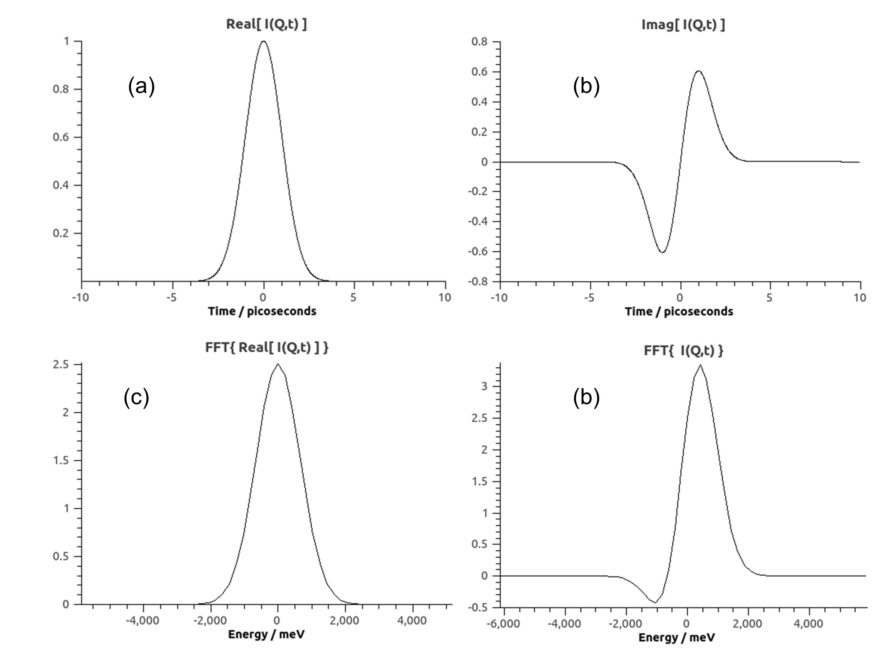
SassenaFFTexample.jpg#
Usage#
Example - Load a Sassena file, Fourier transform it, and do a fit of S(Q,E):
ws = LoadSassena("loadSassenaExample.h5", TimeUnit=1.0)
SassenaFFT(ws, FFTonlyRealPart=1, Temp=1000, DetailedBalance=1)

print('workspaces instantiated:  {}'.format(', '.join(ws.getNames())))

sqt = ws[3] # S(Q,E)
# I(Q,t) is a Gaussian, thus S(Q,E) is a Gaussian too (at high temperatures)
# Let's fit it to a Gaussian. We start with an initial guess
intensity = 100.0
center = 0.0
sigma = 0.01    #in meV
startX = -0.1   #in meV
endX = 0.1
myFunc = 'name=Gaussian,Height={0},PeakCentre={1},Sigma={2}'.format(intensity,center,sigma)

# Call the Fit algorithm and perform the fit
fit_output = Fit(Function=myFunc, InputWorkspace=sqt, WorkspaceIndex=0,
                 StartX = startX, EndX=endX, Output='fit')
paramTable = fit_output.OutputParameters  # table containing the optimal fit parameters
fitWorkspace = fit_output.OutputWorkspace

print("The fit was: " + str(fit_output.OutputStatus))
print("Fitted Height value is: {:.1f}".format(paramTable.column(1)[0]))
print("Fitted centre value is: {:.1f}".format(abs(paramTable.column(1)[1])))
print("Fitted sigma value is: {:.4f}".format(paramTable.column(1)[2]))
# fitWorkspace contains the data, the calculated and the difference patterns
print("Number of spectra in fitWorkspace is: " +  str(fitWorkspace.getNumberHistograms()))
Output:
workspaces instantiated:  ws_qvectors, ws_fqt.Re, ws_fqt.Im, ws_sqw
The fit was: success
Fitted Height value is: 250.7
Fitted centre value is: 0.0
Fitted sigma value is: 0.0066
Number of spectra in fitWorkspace is: 3
Categories: AlgorithmIndex | Arithmetic\FFT
Source#
C++ header: SassenaFFT.h
C++ source: SassenaFFT.cpp