DGS Planner#
Overview#
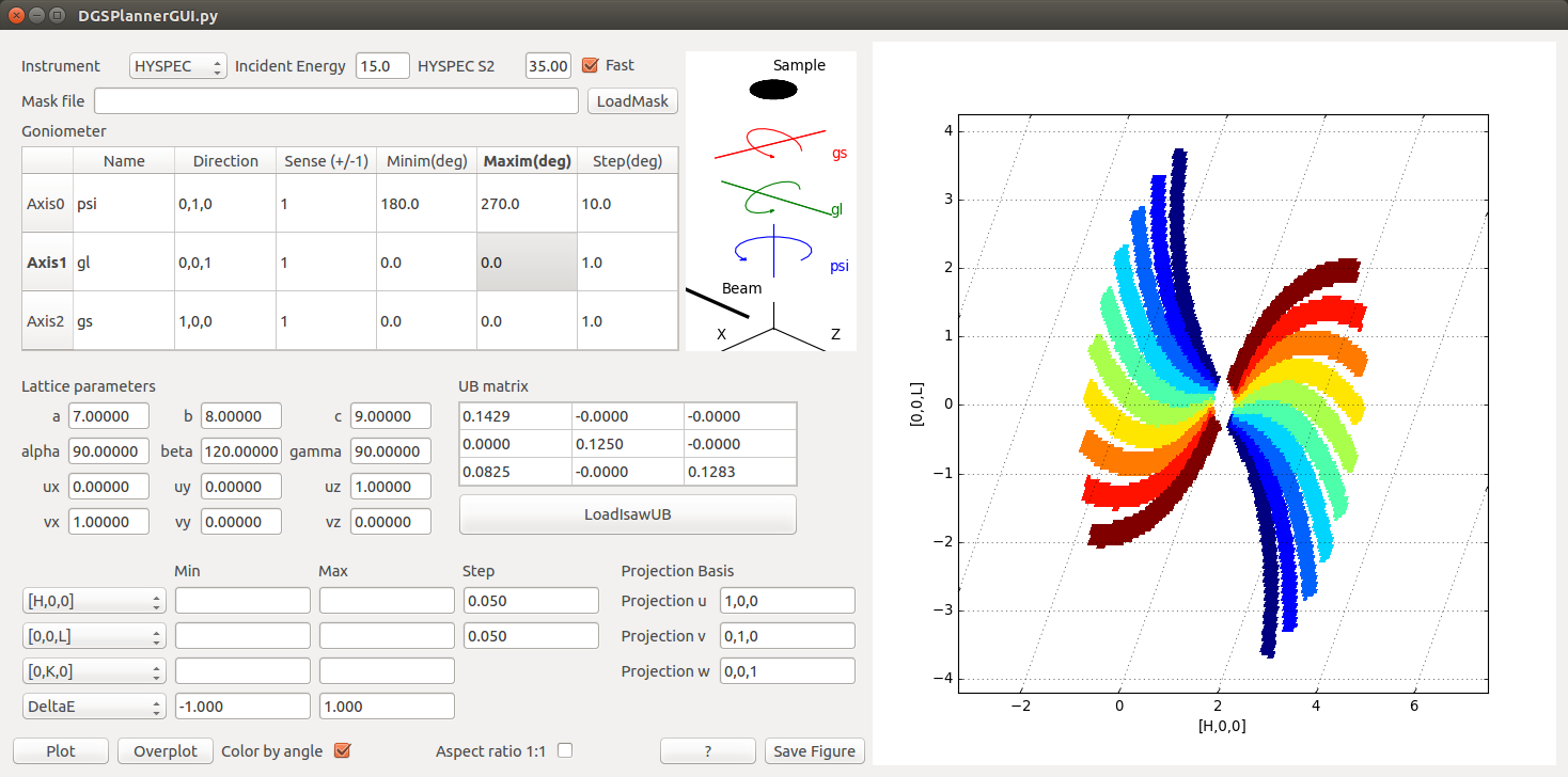
DGSPlanner is an interface for plotting expected coverage for direct geometry time-of-flight instruments. It is based on the CalculateCoverageDGS algorithm.
Instrument options#
One can select an Instrument from the list. Please contact the Mantid developer team to add more options. The latest instrument geometry is loaded from the instrument definition file. In the case of HYSPEC, a value for the S2 angle is required. The monochromator to sample distance is chosen to be msd=1798.5. The Incident Energy is in mili-electron-Volts. The Fast option will use only 25% of the detectors to calculate the coverage. One can use a previously saved Mantid workspace containing a mask, the Mask file option, to eliminate from the coverage calculations detectors that are masked in the experiment.
For the constant wavelength instrument WAND² there are options for S2 and DetZ values to move the detector, the incident energy is changed to wavelength and the DeltaE is fixed to ±1%.
The Goniometer settings follow the Mantid convention (see SetGoniometer. The default values follow the goniometer description in Horace. The name of the axis is just used for plotting. z direction (0,0,1) is along the beam, y direction (0,1,0) is pointing vertically upward, and the x direction (1,0,0) is in the horizontal plane, perpendicular to z. The Sense is either 1 for counterclockwise rotations, or -1 for clockwise rotation. The minimum, maximum, and step values for each goniometer axis describe all sample positions for which the trajectories calculation are made. If more than 10 orientations are selected, the user will be promted to proceed, since this might take longer.
Sample settings#
Information about the sample can be introduced either in terms of Lattice parameters and orientation vectors, or the UB matrix. One can also load an ISAW UB matrix or load the UB matrix from the Nexus metadata. For more information, look at SetUB
Viewing axes#
The default projection axes are [H,0,0], [0,K,0], [0,0,L], and DeltaE. One can modify the momentum transfer components by changing the Projection Basis. Modifying these values will automatically change the viewing axes labels on the left. For example, if Projection u is 1,1,1, the first label on the left side is going to be [H,H,H].
The first viewing axis is going to be the x axis of the plot, the second is the y axis. One can choose an integration range in the other two directions. When swapping viewing axes, the program remembers settings for minimum, maximum, and step.
Note
If the angle between the x and y viewing axes is not 90 degrees, the plot will have non-orthogonal axes
Plotting#
Clicking on the Plot button will generate a plot of the coverage for the selected instrument, for all the goniometer settings. One can Overplot a different configuration (goniometer setting, incident energy, or instrument). If the lattice parameters are different, or the projection basis / viewing axes have changed, the Overplot will just automatically revert to Plot. If Color by angle option is selected, each goniometer setting will have a different color. The blue indicates lower first angle.
In some case, for example when sample has a hexagonal lattice, one might wish to use the Aspect ratio 1:1 option, which would force the x and y to have the same lengths. Please do not use it if one of the axis is DeltaE, since this can yield very elongated figures.
The ? button will show this help page.
The Save Figure button will save the image on the right, and information about the instrument, goniometer, sample, and integration limits into a png file.
Category: Interfaces