Step Scan Analysis#
Interface Overview#
The step scan analysis graphical interface is a simple tool for the analysis of scan runs taken primarily on ADARA-enabled beamlines at the SNS. As the name suggests, it is for the analysis of stepping scans (a.k.a. rocking curves) rather than, e.g., continuous rotation runs and relies on the scan index markers included in the logs to allow the splitting of a single run into the separate scan points. It uses the StepScan algorithm to perform most of the work.
Basic Offline Usage#
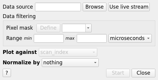
The first step is to load the run to be analysed, which can be accomplished via either the Browse button or, if the file is in your search path, by entering the run number (prefixed with the instrument name if not your default instrument). The file will immediately load and enable the controls to run the analysis. The drop-down list of variables to plot against will be populated with all of the logs which changed value during the run. You will need to select the variable that you were scanning against, or can just plot against scan_index. The normalization options are: none, time, the summed proton charge in the step or the counts in any monitors that have been loaded.
Hitting Start will run the StepScan algorithm and generate the rocking curve plot (see example screenshot below). The plot variable and normalization can be interactively changed via the drop-down lists. When you are done, pressing Close will close the plot and remove all workspaces apart from the table. Choosing a different file (or the live button - see below) will do the same, but also load the new data which can be analysed by once more clicking Start.
Region of Interest Selection#
The data included in the analysis can be refined via the controls in the Data filtering section of the interface. A pixel mask can be given either by selecting a previously loaded/generated masking workspace or by clicking Define, which will launch the Instrument View window. From there, you can draw your region of interest and save it to a workspace via Apply and Save followed by As ROI to workspace. The generated workspace (called MaskWorkspace) will be automatically selected for the Pixel mask option. You can also filter by time (later, other units will be added) by entering minimum and maximum values in the boxes provided.
Analyzing Scans from Pre-ADARA Data Files#
Step scans where each scan point is saved to a separate file (e.g. a simple PyDas scan where ‘save_events’ was set to true). If multiple event nexus files are given as the data source then they will be loaded and then combined after a sequential scan index marker has been inserted into each run. They can then be analyzed in the normal way.
Live Usage#
If, on starting the interface, the ability to connect to the live data feed of your
default instrument is detected, then the Use live stream button will become enabled.
This needs to be an ADARA-enabled SNS beamline.
Selecting the button will start data collection and continuously update the
Plot against drop-down with any variables which change during the run
(scan_index will always be present).
Hitting start will generate the plot, which will then auto-update as the run progresses.
Live data collection will stop when the end of the run is detected.
Note: Start should only be clicked once the scan run has started.
Categories: Interfaces | General