Exercises#
Part 1#
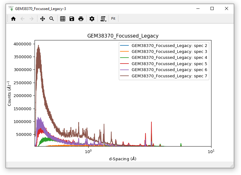
Load the File “GEM38370_Focussed_Legacy.nxs”.
Plot spectra 2-7 (all of them).
Edit the d-spacing axis range to 0.01-10 Å.
Try changing the X-Axis Scale to Symlog.
Part 2#
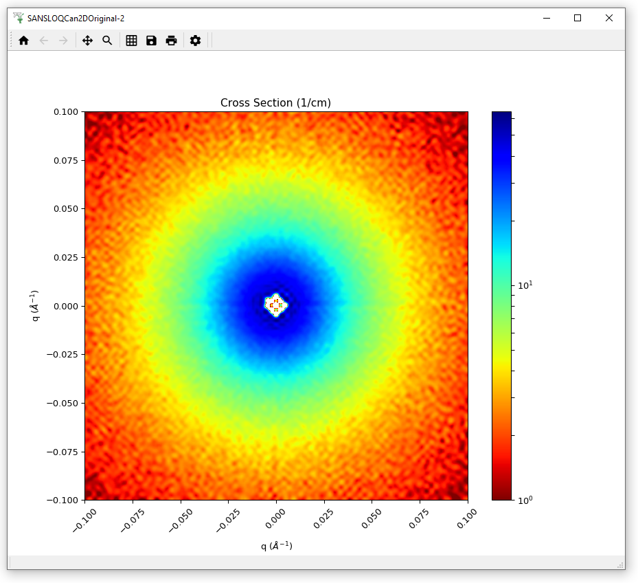
Load the SANSLOQCan2D.nxs data. This is the output of a 2D SANS data reduction. Although a Workspace2D is mainly designed to store spectra, this is just the default, and in this data the loaded axes are momentum transfer Qx and the scattering cross section, and the ‘spectrum’ axis is momentum transfer Qy.
Plot this data as a colour fill plot.
Change the Image/Colour bar Scale to Logarithmic.
Change the Colour Map to Jet and reverse it.
Set the Min. value of the Image/Color bar to 1.
Change the Interpolation to “Sinc”.
Part 3#
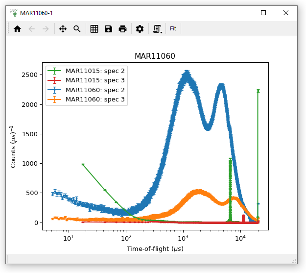
Using the workspaces MAR11015 and MAR11060 try to reproduce the plot below. Note it contains spectra 2 and 3 of both Workspaces
You must either Plot and then Overplot, or Group the Workspaces before plotting: try both!
Then adjust the axes to use log(x), linear(y) scaling
I have also Applied to All curves a size 4 point Marker and Error bars with Capsize 2, which can be done in Figure Options.
As a bonus part. Click the ‘Generate a Script’ button in the Plot Toolbar and save this script to file as “My_MARI_Plot.py”. Close this plot and in the main Mantid window, select “File > Open Script” and navigate to your saved script. This script will open in the “Editor” window.
Use of Python within Mantid is saved for a follow-up course as it is not required, but here is a little preview of how it can be used, and more importantly how you can create a useful script for producing a plot!
Now you’ve got the script loaded, click the green arrow button to run this script, and your plot will appear!