Python in Mantid: Solution 3#
All the data for these solutions can be found in the TrainingCourseData on the Downloads page.
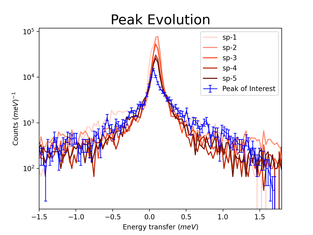
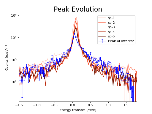
A - Direct Matplotlib with SNS Data#
# import mantid algorithms, numpy and matplotlib
from mantid.simpleapi import *
import matplotlib.pyplot as plt
import numpy as np

# Load the data
run = Load('Training_Exercise3a_SNS.nxs')

fig, axes = plt.subplots(subplot_kw={'projection': 'mantid'})

# Choose legend labels and colors for each curve
labels = ("sp-1", "sp-2", "sp-3", "sp-4", "sp-5")
colors = ('#FFCFC4', '#FE886F','#FE4A23', '#B82405', '#6A1300')

# Plot the first 5 spectra
for i in range(5):
    axes.plot(run, wkspIndex=i, color=colors[i], label=labels[i])

# Plot the 9th spectrum with errorbars
axes.errorbar(run, specNum=9, capsize=2.0, color='blue', label='Peak of Interest', linewidth=1.0)

# Set the X-axis limts and the Y-axis scale
axes.set_xlim(-1.5, 1.8)
plt.yscale('log')

# Give the plot a title
plt.title("Peak Evolution", fontsize=20)

# Add a legend with the chosen labels and show the plot
axes.legend()
#fig.show() #uncomment to show the plot

# Note with the Direct Matplotlib method,
# there are many more options for formatting the plot
(Source code, png, hires.png, pdf)
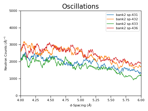
B - plotSpectrum with ISIS Data#
# import mantid algorithms, numpy and matplotlib
from mantid.simpleapi import *
import matplotlib.pyplot as plt
import numpy as np
from mantid.plots._compatability import plotSpectrum #import needed outside Workbench

'''Processing'''

# Load the spectral range of the interest of the data
ws=Load(Filename="GEM40979.raw", SpectrumMin=431, SpectrumMax=750)

# Convert to dSpacing
ws=ConvertUnits(InputWorkspace=ws, Target= "dSpacing")

# Smooth the data
ws=SmoothData(InputWorkspace=ws, NPoints=20)

'''Plotting'''

# Plot three spectra
PLOT_WINDOW = plotSpectrum(ws, [0,1,2])

# Get Figure and Axes for formatting
fig, axes = plt.gcf(), plt.gca()

# Set the scales on the x- and y-axes
axes.set_xlim(4, 6)
axes.set_ylim(0, 5e3)

# Plot index 5
plotSpectrum(ws,5, window= PLOT_WINDOW, clearWindow= False)

# Alter the Y label
axes.set_ylabel('Neutron Counts ($\AA$)$^{-1}$')

# Optionally rename the curve titles
axes.legend(["bank2 sp-431", "bank2 sp-432", "bank2 sp-433", "bank2 sp-436"])

# Give the plot a title
plt.title("Oscillations", fontsize=20)
(Source code, png, hires.png, pdf)

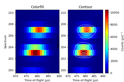
C - 2D and 3D Plot ILL Data#
# import mantid algorithms, numpy and matplotlib
from mantid.simpleapi import *
import matplotlib.pyplot as plt
import numpy as np
# Load the data and extract the region of interest
data=Load('164198.nxs')
data=ExtractSpectra(data, XMin=470, XMax=490, StartWorkspaceIndex=199, EndWorkspaceIndex=209)
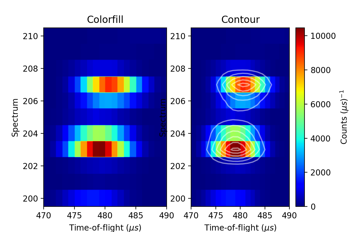
'''2D Plotting - Colorfill and Contour'''
# Get a figure and axes for
figC,axC = plt.subplots(ncols=2, subplot_kw={'projection':'mantid'}, figsize = (6,4))
# Plot the data as a 2D colorfill: IMPORTANT to set origin to lower
c=axC[0].imshow(data,cmap='jet', aspect='auto', origin = 'lower')
# Change the title
axC[0].set_title("Colorfill")
# Plot the data as a 2D colorfill: IMPORTANT to set origin to lower
c=axC[1].imshow(data,cmap='jet', aspect='auto', origin = 'lower')
# Overlay Contour lines
axC[1].contour(data, levels=np.linspace(0, 10000, 7), colors='white', alpha=0.5)
# Change the title
axC[1].set_title("Contour")
# Add a Colorbar with a label
cbar=figC.colorbar(c)
cbar.set_label(r'Counts ($\mu s$)$^{-1}$')
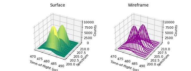
'''3D Plotting - Surface and Wireframe'''
# Get a different set of figure and axes with 3 subplots for 3D plotting
fig3d,ax3d = plt.subplots(ncols=2, subplot_kw={'projection':'mantid3d'}, figsize = (8,3))
# 3D plot the data, and choose colormaps and colors
ax3d[0].plot_surface(data, cmap='summer')
ax3d[1].plot_wireframe(data, color='darkmagenta')
# Add titles to the 3D plots
ax3d[0].set_title("Surface")
ax3d[1].set_title("Wireframe")
#figC.show()# uncomment to show the plots
#fig3d.show()