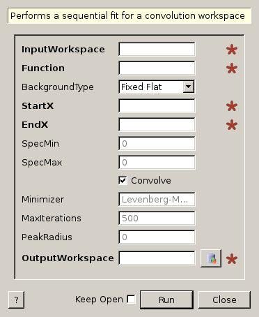
ConvolutionFitSequential dialog.
Table of Contents
| Name | Direction | Type | Default | Description |
|---|---|---|---|---|
| InputWorkspace | Input | MatrixWorkspace | Mandatory | The input workspace for the fit. |
| Function | Input | string | Mandatory | The function that describes the parameters of the fit. |
| BackgroundType | Input | string | Fixed Flat | The Type of background used in the fitting. Allowed values: [‘Fixed Flat’, ‘Fit Flat’, ‘Fit Linear’] |
| StartX | Input | number | Mandatory | The start of the range for the fit function. |
| EndX | Input | number | Mandatory | The end of the range for the fit function. |
| SpecMin | Input | number | 0 | The first spectrum to be used in the fit. Spectra values can not be negative |
| SpecMax | Input | number | 0 | The final spectrum to be used in the fit. Spectra values can not be negative |
| Convolve | Input | boolean | True | If true, the fit is treated as a convolution workspace. |
| Minimizer | Input | string | Levenberg-Marquardt | Minimizer to use for fitting. Minimizers available are ‘Levenberg-Marquardt’, ‘Simplex’, ‘FABADA’, ‘Conjugate gradient (Fletcher-Reeves imp.)’, ‘Conjugate gradient (Polak-Ribiere imp.)’ and ‘BFGS’ |
| MaxIterations | Input | number | 500 | The maximum number of iterations permitted |
| PeakRadius | Input | number | 0 | A value of the peak radius the peak functions should use. A peak radius defines an interval on the x axis around the centre of the peak where its values are calculated. Values outside the interval are not calculated and assumed zeros.Numerically the radius is a whole number of peak widths (FWHM) that fit into the interval on each side from the centre. The default value of 0 means the whole x axis. |
| OutputWorkspace | Output | MatrixWorkspace | Mandatory | The OutputWorkspace containing the results of the fit. |
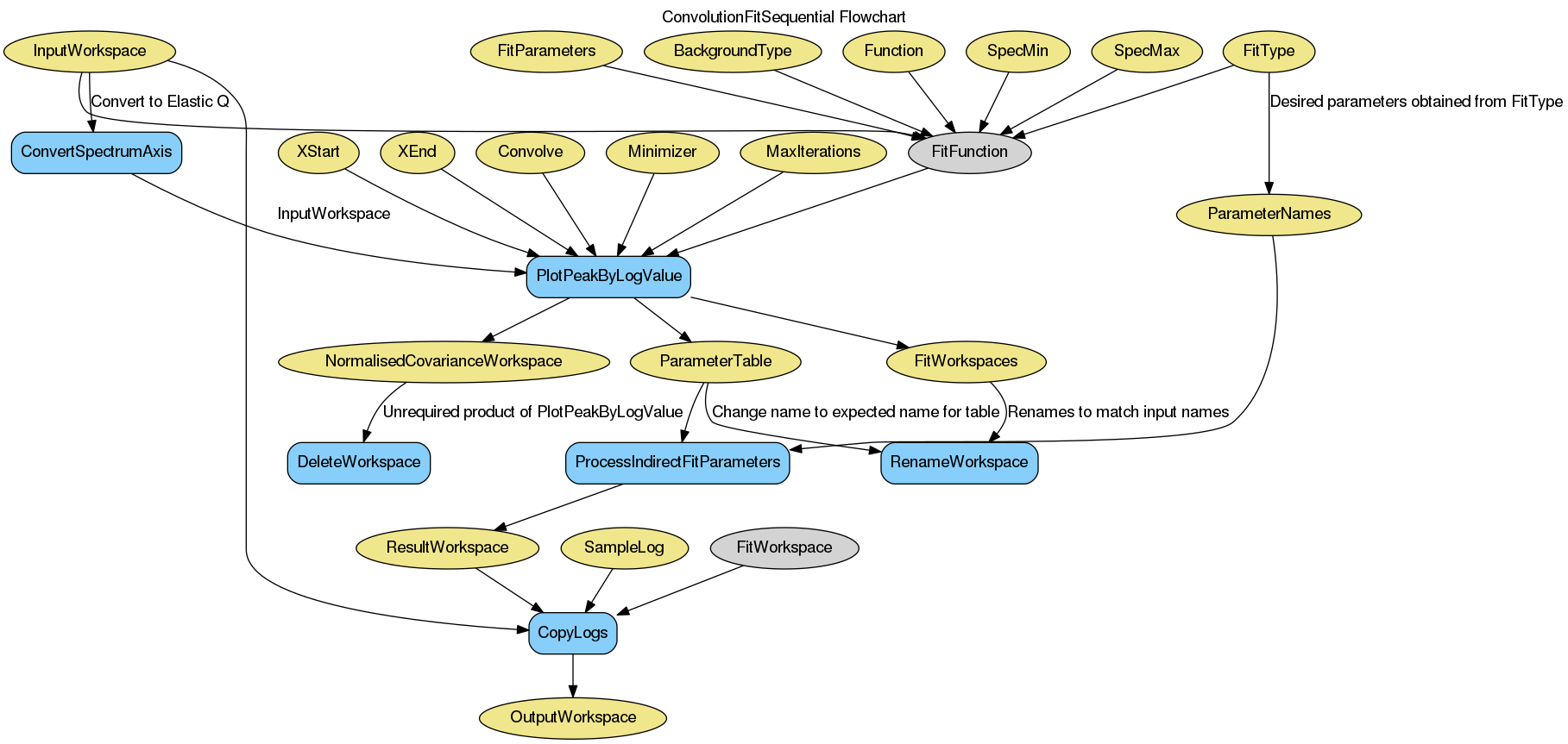
An algorithm designed mainly as a sequential call to PlotPeakByLogValue but used within the ConvFit tab within the Indirect Analysis interface to fit Convolution Functions.
Example - ConvolutionFitSequential
# Create a host workspace
sample = Load('irs26176_graphite002_red.nxs')
resolution = Load('irs26173_graphite002_red.nxs')

# Set up algorithm parameters
function = "name=LinearBackground,A0=0,A1=0,ties=(A0=0.000000,A1=0.0);(composite=Convolution,FixResolution=true,NumDeriv=true;name=Resolution,Workspace=__ConvFit_Resolution,WorkspaceIndex=0;((composite=ProductFunction,NumDeriv=false;name=Lorentzian,Amplitude=1,PeakCentre=0,FWHM=0.0175)))"
bgType = "Fixed Flat"
startX = -0.547608
endX = 0.543217
specMin = 0
specMax = sample.getNumberHistograms() - 1
convolve = True
minimizer = "Levenberg-Marquardt"
maxIt = 500

# Build resolution workspace (normally done by the Convfit tab when files load)
AppendSpectra(InputWorkspace1=resolution.name(), InputWorkspace2=resolution.name(), OutputWorkspace="__ConvFit_Resolution")
for i in range(1, sample.getNumberHistograms()):
  AppendSpectra(InputWorkspace1="__ConvFit_Resolution", InputWorkspace2=resolution.name(), OutputWorkspace="__ConvFit_Resolution")

# Run algorithm
result_ws = ConvolutionFitSequential(InputWorkspace=sample, Function=function ,BackgroundType=bgType, StartX=startX, EndX=endX, SpecMin=specMin, SpecMax=specMax, Convolve=convolve, Minimizer=minimizer, MaxIterations=maxIt)

print "Result has %i Spectra" %result_ws.getNumberHistograms()

print "Amplitude 0: %.3f" %(result_ws.readY(0)[0])
print "Amplitude 1: %.3f" %(result_ws.readY(0)[1])
print "Amplitude 2: %.3f" %(result_ws.readY(0)[2])

print "X axis at 0: %.5f" %(result_ws.readX(0)[0])
print "X axis at 1: %.5f" %(result_ws.readX(0)[1])
print "X axis at 2: %.5f" %(result_ws.readX(0)[2])

print "Amplitude Err 0: %.5f" %(result_ws.readE(0)[0])
print "Amplitude Err 1: %.5f" %(result_ws.readE(0)[1])
print "Amplitude Err 2: %.5f" %(result_ws.readE(0)[2])
Output:
Result has 2 Spectra

Amplitude 0: 4.314
Amplitude 1: 4.179
Amplitude 2: 3.979

X axis at 0: 0.52531
X axis at 1: 0.72917
X axis at 2: 0.92340

Amplitude Err 0: 0.00460
Amplitude Err 1: 0.00464
Amplitude Err 2: 0.00504
Categories: Algorithms | Workflow\MIDAS