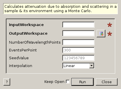
MonteCarloAbsorption v1¶

MonteCarloAbsorption dialog.

Table of Contents

Summary
Properties
Description
Usage
References
Source

Summary ¶

Calculates attenuation due to absorption and scattering in a sample & its environment using a Monte Carlo.

Properties ¶

Name	Direction	Type	Default	Description
InputWorkspace	Input	MatrixWorkspace	Mandatory	The name of the input workspace. The input workspace must have X units of wavelength.
OutputWorkspace	Output	MatrixWorkspace	Mandatory	The name to use for the output workspace.
NumberOfWavelengthPoints	Input	number	Optional	The number of wavelength points for which a simulation is atttempted (default: all points)
EventsPerPoint	Input	number	300	The number of “neutron” events to generate per simulated point
SeedValue	Input	number	123456789	Seed the random number generator with this value
Interpolation	Input	string	Linear	Method of interpolation used to compute unsimulated values. Allowed values: [‘Linear’, ‘CSpline’]

Description ¶

This algorithm performs a Monte Carlo simulation to calculate the correction factors due to attenuation & single scattering within a sample plus optionally its sample environment.

Input Workspace Requirements ¶

The algorithm will compute the correction factors on a bin-by-bin basis for each spectrum within the input workspace. The following assumptions on the input workspace will are made:

X units are in wavelength
the instrument is fully defined
properties of the sample and optionally its environment have been set with SetSample

By default the beam is assumed to be the a slit with width and height matching the width and height of the sample. This can be overridden using SetBeam.

By default, the material for the sample & containers will define the values of the cross section used to compute the absorption factor and will include contributions from both the total scattering cross section & absorption cross section. This follows the Hamilton-Darwin [1], [2] approach as described by T. M. Sabine in the International Tables of Crystallography Vol. C [3].

The algorithm proceeds as follows. For each spectrum:

find the associated detector position
find the associated efixed value (if applicable) & convert to wavelength ( $\lambda_{fixed}$ )
loop over the bins in steps defined by NumberOfWavelengthPoints and for each step ()
- define as the wavelength before scattering & as wavelength after scattering:
  - Direct: $\lambda_1 = \lambda_1$ , $\lambda_2 = \lambda_{step}$
  - Indirect: $\lambda_1 = \lambda_{step}$ , $\lambda_2 = \lambda_{fixed}$
  - Elastic: $\lambda_1 = \lambda_2 = \lambda_{step}$
- for each event in NEvents:
  - generate a random point on the beam face defined by the input height & width. If the point is outside of the area defined by the face of the sample then it is pulled to the boundary of this area
  - generate a random point within the sample or container objects as the scatter point and create a Track from the selected position on the beam face to the scatter point
  - test for intersections of the track & sample/container objects, giving the number of subsections and corresponding distances within the object for each section, call them $l_{1i}$
  - form a second Track with the scatter position as the starting point and the direction defined by detPos - scatterPos
  - test for intersections of the track & sample/container objects, giving the number of subsections and corresponding distances within the object for each section, call them $l_{2i}$
  - compute the self-attenuation factor for all intersections as $\prod\limits_{i} \exp(-(\rho_{1i}\sigma_{1i}(\lambda_{1i})l_{1i} + \rho_{2i}\sigma_{2i}(\lambda_{2i})l_{2i}))$ where $\rho$ is the mass density of the material & $\sigma$ the absorption cross-section at a given wavelength
  - accumulate this factor with the factor for all NEvents
- average the accumulated attentuation factors over NEvents and assign this as the correction factor for this $\lambda_{step}$ .
finally, interpolate through the unsimulated wavelength points using the selected method

Interpolation ¶

The default linear interpolation method will produce an absorption curve that is not smooth. CSpline interpolation will produce a smoother result by using a 3rd-order polynomial to approximate the original points.

Usage ¶

Example: A cylindrical sample with no container

data = CreateSampleWorkspace(WorkspaceType='Histogram', NumBanks=1)
data = ConvertUnits(data, Target="Wavelength")
# Default up axis is Y
SetSample(data, Geometry={'Shape': 'Cylinder', 'Height': 5.0, 'Radius': 1.0,
                  'Center': [0.0,0.0,0.0]},
                Material={'ChemicalFormula': '(Li7)2-C-H4-N-Cl6', 'SampleNumberDensity': 0.07})
# Simulating every data point can be slow. Use a smaller set and interpolate
abscor = MonteCarloAbsorption(data, NumberOfWavelengthPoints=50)
corrected = data/abscor

Example: A cylindrical sample with no container, interpolating with a CSpline

data = CreateSampleWorkspace(WorkspaceType='Histogram', NumBanks=1)
data = ConvertUnits(data, Target="Wavelength")
# Default up axis is Y
SetSample(data, Geometry={'Shape': 'Cylinder', 'Height': 5.0, 'Radius': 1.0,
                  'Center': [0.0,0.0,0.0]},
                Material={'ChemicalFormula': '(Li7)2-C-H4-N-Cl6', 'SampleNumberDensity': 0.07})
# Simulating every data point can be slow. Use a smaller set and interpolate
abscor = MonteCarloAbsorption(data, NumberOfWavelengthPoints=50,
                              Interpolation='CSpline')
corrected = data/abscor

Example: A cylindrical sample setting a beam size

data = CreateSampleWorkspace(WorkspaceType='Histogram', NumBanks=1)
data = ConvertUnits(data, Target="Wavelength")
# Default up axis is Y
SetSample(data, Geometry={'Shape': 'Cylinder', 'Height': 5.0, 'Radius': 1.0,
                  'Center': [0.0,0.0,0.0]},
                  Material={'ChemicalFormula': '(Li7)2-C-H4-N-Cl6', 'SampleNumberDensity': 0.07})
SetBeam(data, Geometry={'Shape': 'Slit', 'Width': 0.8, 'Height': 1.0})
# Simulating every data point can be slow. Use a smaller set and interpolate
abscor = MonteCarloAbsorption(data, NumberOfWavelengthPoints=50)
corrected = data/abscor

Example: A cylindrical sample with predefined container

The following example uses a test sample environment defined for the TEST_LIVE facility and ISIS_Histogram instrument and assumes that these are set as the default facility and instrument respectively. The definition can be found at [INSTALLDIR]/instrument/sampleenvironments/TEST_LIVE/ISIS_Histogram/CRYO-01.xml.

data = CreateSampleWorkspace(WorkspaceType='Histogram', NumBanks=1)
data = ConvertUnits(data, Target="Wavelength")
# Sample geometry is defined by container but not completely filled so
# we just define the height
SetSample(data, Environment={'Name': 'CRYO-01', 'Container': '8mm'},
          Geometry={'Height': 4.0},
          Material={'ChemicalFormula': '(Li7)2-C-H4-N-Cl6', 'SampleNumberDensity': 0.07})
# Simulating every data point can be slow. Use a smaller set and interpolate
abscor = MonteCarloAbsorption(data, NumberOfWavelengthPoints=30)
corrected = data/abscor

References ¶

[1]	Darwin, C. G., Philos. Mag., 43 800 (1922) doi: 10.1080/10448639208218770

[2]	Hamilton, W.C., Acta Cryst, 10, 629 (1957) doi: 10.1107/S0365110X57002212

[3]	Sabine, T. M., International Tables for Crystallography, Vol. C, Page 609, Ed. Wilson, A. J. C and Prince, E. Kluwer Publishers (2004) doi: 10.1107/97809553602060000103

Categories: Algorithms | CorrectionFunctions\AbsorptionCorrections

Source ¶

C++ source: MonteCarloAbsorption.cpp

C++ header: MonteCarloAbsorption.h