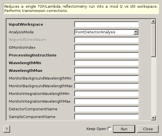
ReflectometryReductionOne v1¶

ReflectometryReductionOne dialog.

Table of Contents

Summary
Properties
Description
High-Level Workflow
Low-Level Workflow
Usage
Source

Summary ¶

Reduces a single TOF/Lambda reflectometry run into a mod Q vs I/I0 workspace. Performs transmission corrections.

Properties ¶

Name	Direction	Type	Default	Description
InputWorkspace	Input	MatrixWorkspace	Mandatory	Run to reduce.
AnalysisMode	Input	string	PointDetectorAnalysis	The type of analysis to perform. Point detector or multi detector. Allowed values: [‘PointDetectorAnalysis’, ‘MultiDetectorAnalysis’]
RegionOfDirectBeam	Input	int list		Indices of the spectra a pair (lower, upper) that mark the ranges that correspond to the direct beam in multi-detector mode.
I0MonitorIndex	Input	number	Optional	I0 monitor workspace index
ProcessingInstructions	Input	string	Mandatory	Grouping pattern on workspace indexes to yield only the detectors of interest. See GroupDetectors for details.
WavelengthMin	Input	number	Mandatory	Wavelength minimum in angstroms
WavelengthMax	Input	number	Mandatory	Wavelength maximum in angstroms
MonitorBackgroundWavelengthMin	Input	number	Optional	Wavelength minimum for monitor background in angstroms.
MonitorBackgroundWavelengthMax	Input	number	Optional	Wavelength maximum for monitor background in angstroms.
MonitorIntegrationWavelengthMin	Input	number	Optional	Wavelength minimum for integration in angstroms.
MonitorIntegrationWavelengthMax	Input	number	Optional	Wavelength maximum for integration in angstroms.
DetectorComponentName	Input	string		Name of the detector component i.e. point-detector. If these are not specified, the algorithm will attempt lookup using a standard naming convention.
SampleComponentName	Input	string		Name of the sample component i.e. some-surface-holder. If these are not specified, the algorithm will attempt lookup using a standard naming convention.
OutputWorkspace	Output	MatrixWorkspace	Mandatory	Output Workspace IvsQ.
OutputWorkspaceWavelength	Output	MatrixWorkspace		Output Workspace IvsLam. Intermediate workspace.
ThetaIn	Input	number	Optional	Final theta value in degrees. Optional, this value will be calculated internally and provided as ThetaOut if not provided.
ThetaOut	Output	number		Calculated final theta in degrees.
NormalizeByIntegratedMonitors	Input	boolean	True	Normalize by dividing by the integrated monitors.
CorrectDetectorPositions	Input	boolean	True	Correct detector positions using ThetaIn (if given)
FirstTransmissionRun	Input	MatrixWorkspace		First transmission run, or the low wavelength transmission run if SecondTransmissionRun is also provided.
SecondTransmissionRun	Input	MatrixWorkspace		Second, high wavelength transmission run. Optional. Causes the FirstTransmissionRun to be treated as the low wavelength transmission run.
Params	Input	dbl list		A comma separated list of first bin boundary, width, last bin boundary. These parameters are used for stitching together transmission runs. Values are in wavelength (angstroms). This input is only needed if a SecondTransmission run is provided.
StartOverlap	Input	number	Optional	Start wavelength for stitching transmission runs together
EndOverlap	Input	number	Optional	End wavelength (angstroms) for stitching transmission runs together
StrictSpectrumChecking	Input	boolean	True	Enforces spectrum number checking prior to normalization
CorrectionAlgorithm	Input	string	None	The type of correction to perform. Allowed values: [‘None’, ‘PolynomialCorrection’, ‘ExponentialCorrection’]
Polynomial	Input	dbl list		Coefficients to be passed to the PolynomialCorrection algorithm.
C0	Input	number	0	C0 value to be passed to the ExponentialCorrection algorithm.
C1	Input	number	0	C1 value to be passed to the ExponentialCorrection algorithm.
ScaleFactor	Input	number	Optional	Factor you wish to scale Q workspace by.
MomentumTransferMinimum	Input	number	Optional	Minimum Q value in IvsQ Workspace. Used for Rebinning the IvsQ Workspace
MomentumTransferStep	Input	number	Optional	Resolution value in IvsQ Workspace. Used for Rebinning the IvsQ Workspace. This value will be made minus to apply logarithmic rebinning. If you wish to have linear bin-widths then please provide a negative DQQ
MomentumTransferMaximum	Input	number	Optional	Maximum Q value in IvsQ Workspace. Used for Rebinning the IvsQ Workspace

Reduces a single TOF reflectometry run into a mod Q vs I/I0 workspace. Performs transmission corrections. Handles both point detector and multidetector cases. The algorithm can correct detector locations based on an input theta value.

Historically the work performed by this algorithm was known as the Quick script.

If MonitorBackgroundWavelengthMin and MonitorBackgroundWavelengthMax are both set to 0, then background normalization will not be performed on the monitors.

The properties of this algorithm should be manually selected by the user. If you wish to use the default values (found in the Instrument Defintion File) for the properties of this algorithm, you may want to consider using ReflectometryReductionOneAuto v2.

ReflectometryReductionOneAuto v2 also performs extra processing steps such as Background subtraction and PolarizationCorrection v1. If you want to know how these processing steps are used, please refer to the ReflectometryReductionOneAuto v2 documentation.

High-Level Workflow ¶

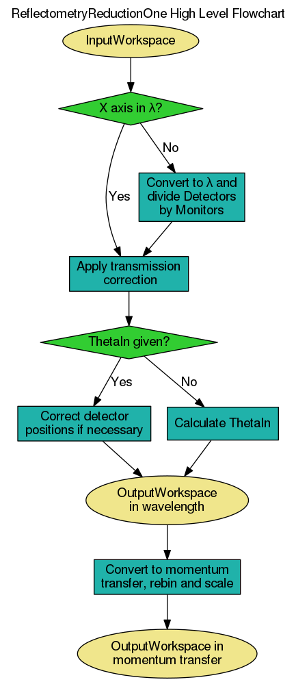
The diagram below displays a high-level version of the algorithm workflow, illustrating the main steps taking place in the ReflectometryReductionOne algorithm. These individual steps are described in more detail in the next sections.

../_images/ReflectometryReductionOne_HighLvl-v1_wkflw.png

Low-Level Workflow ¶

Conversion to Wavelength ¶

The following diagram describes the steps taken in converting the input workspace into units of wavelength and dividing its constituent detectors by monitors.

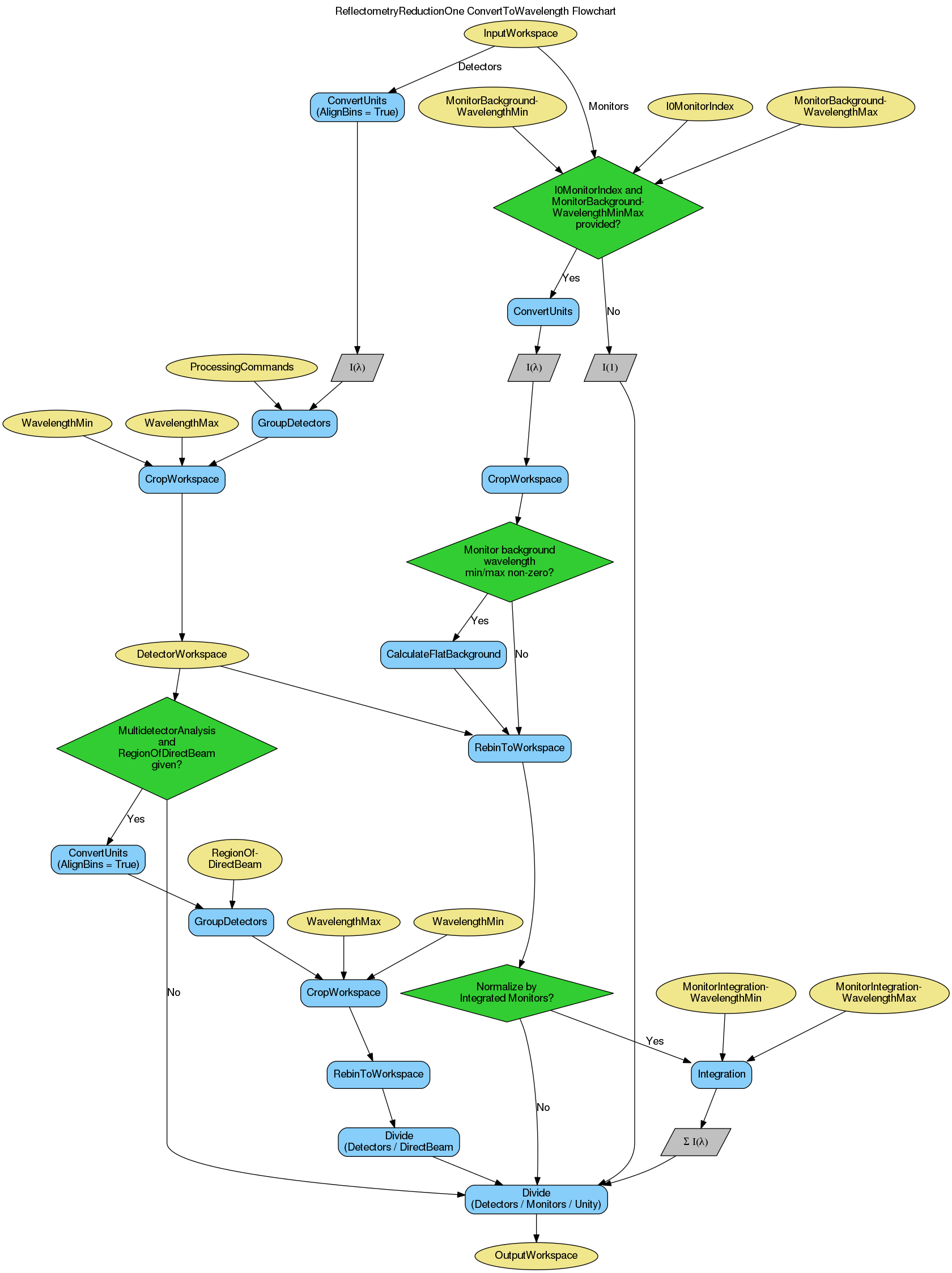
../_images/ReflectometryReductionOne_ConvertToWavelength-v1_wkflw.png

The default analysis mode is PointDetectorAnalysis. For PointAnalysisMode the analysis can be roughly reduced to IvsLam = DetectorWS / sum(I0) / TransmissionWS / sum(I0). For MultiDetectorAnalysis the analysis can be roughly reduced to IvsLam = DetectorWS / RegionOfDirectBeamWS / sum(I0) / TransmissionWS / sum(I0).

Transmission Correction ¶

This diagram shows how the resultant workspace of the previous step is corrected by either by provided transmission runs or by a specific correction algorithm.

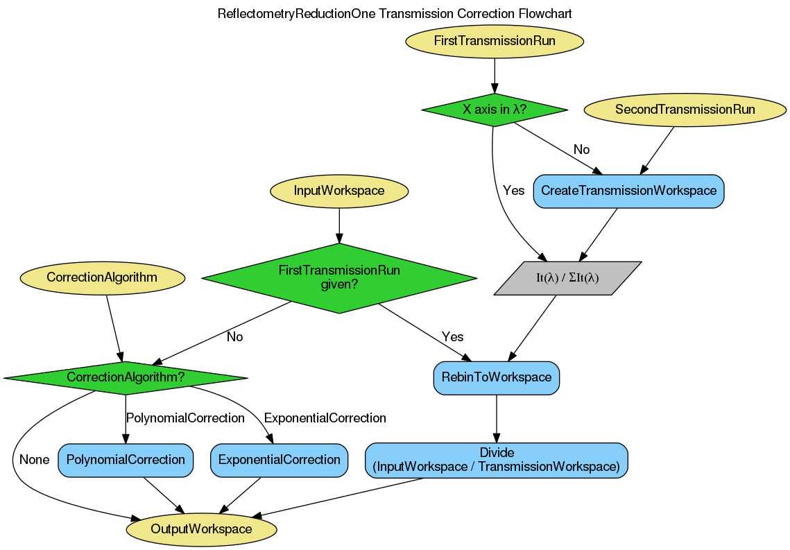
Transmission correction is a normalization step, which may be applied to both PointDetectorAnalysis and MultiDetectorAnalysis reduction.

Transmission runs are expected to be in TOF. The spectra numbers in the Transmission run workspaces must be the same as those in the Input Run workspace. If two Transmission runs are provided then the Stitching parameters associated with the transmission runs will also be required. If a single Transmission run is provided, then no stitching parameters will be needed.

The normalization by tranmission run(s) is optional.

The input workspace provided to the workflow in this instance is the original InputWorkspace after conversion to wavelength and normalization by monitors, as shown in the previous Conversion To Wavelength diagram.

The output workspace given is not the output to the whole algorithm. Rather it will serve as the input workspace to the Polynomial Correction workflow, where further steps will be applied to it.

Polynomial Correction ¶

If no Transmission runs are provided, then polynomial correction can be performed instead. Polynomial correction is enabled by setting the CorrectionAlgorithm property. If set to PolynomialCorrection it runs the PolynomialCorrection v1 algorithm, with this algorithms Polynomial property used as its Coefficients property.

If the CorrectionAlgorithm property is set to ExponentialCorrection, then the ExponentialCorrection v1 algorithm is used, with C0 and C1 taken from the C0 and C1 properties.

Detector Position Correction ¶

The diagram below describes how the input workspace is then corrected by detector positions after transmission correction.

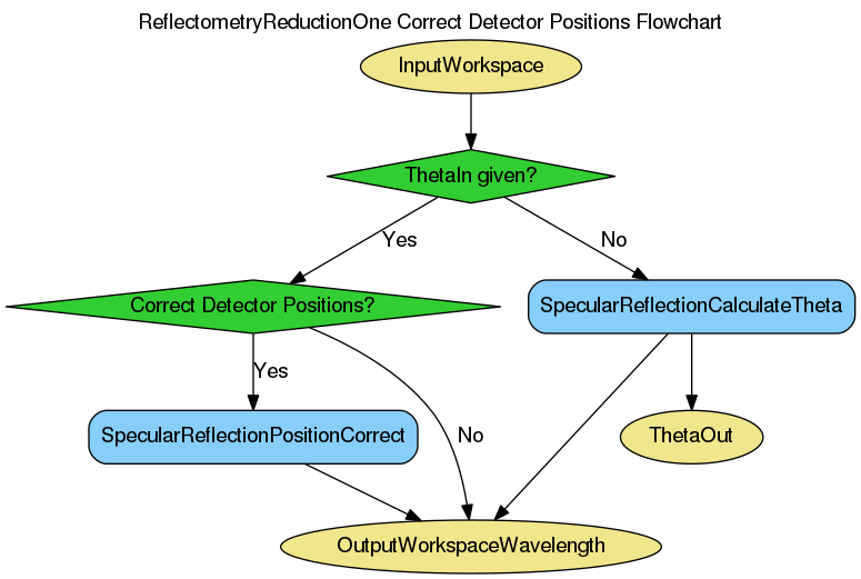
../_images/ReflectometryReductionOne_CorrectDetectorPositions-v1_wkflw.png

Detector Position Correction is used for when the position of the detector is not aligned with the reflected beamline. The correction algorithm used is SpecularReflectionPositionCorrect v1 which is a purely vertical position correction.

The detector positions in this process are corrected in terms of ThetaIn. In general, the detector posistions should always be corrected unless the InputWorkspace already has the detectors in the right positions. This can be achieved by running MoveInstrumentComponent before ReflectometryReductionOne.

Convert To Momentum Transfer (Q)¶

The last diagram describes the steps involved in converting the input workspace from units of wavelength into momentum transfer (Q).

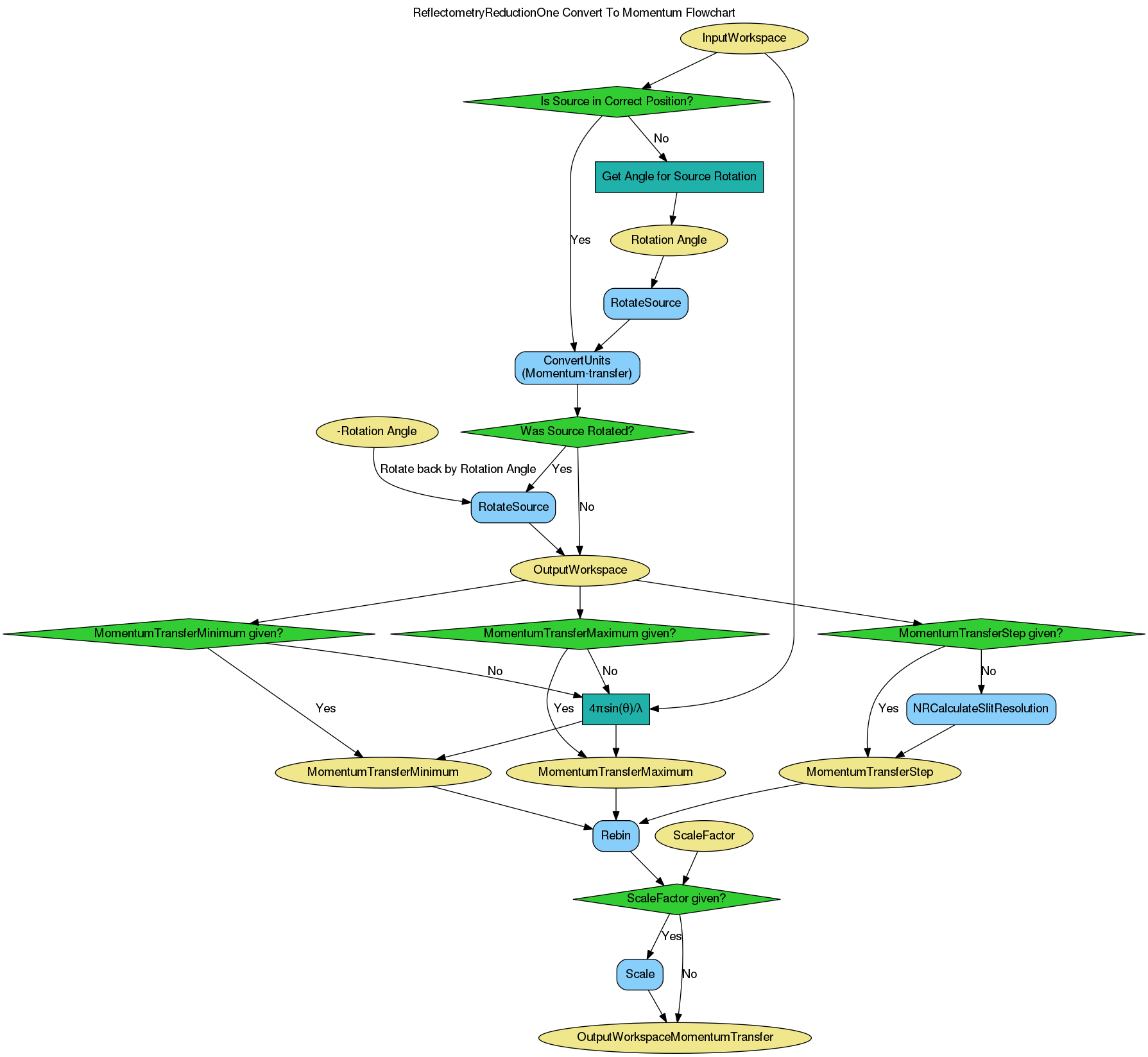
../_images/ReflectometryReductionOne_ConvertToMomentum-v1_wkflw.png

ReflectometryReductionOne contains 2 post-processing options that will be applied to the IvsQ workspace. These two options are Rebin and Scale.

Rebinning ¶

To Rebin your IvsQ workspace you will have to provide values for the following properties: MomentumTransferMinimum, MomentumTransferStep and MomentumTransferMaximum. These values will be appended to each other to form your Rebin v1 Params. These values correspond to your MinimumExtent, BinWidth and MaximumExtent respectively.

If you provide a positive MomentumTransferStep value then the algorithm will automatically negate this value which will allow for Logarithmic Rebinning. Alternatively, a negative MomentumTransferStep will result in Linear Rebinning. More details about the Rebinning process can be found in the documentation for Rebin v1.

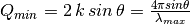
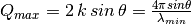
If no values are provided for MomentumTransferMinimum and MomentumTransferMaximum then the algorithm will attempt to calculate these values by using the equations below:

$Q_{min} = 2 \, k \, sin \, \theta = \frac{4 \pi sin \theta}{\lambda_{max}}$

$Q_{max} = 2 \, k \, sin \, \theta = \frac{4 \pi sin \theta}{\lambda_{min}}$

Where $\lambda_{min}$ is the minimum extent of the IvsLambda Workspace and $\lambda_{max}$ is the maximum extent of the IvsLambda Workspace.

If you have not provided a value for MomentumTransferStep then the algorithm will use NRCalculateSlitResolution v1 to calculate this value for you.

Scaling ¶

To apply a scaling to the IvsQ workspace that has been produced by the reduction, you will need to provide a value for the ScaleFactor property in the algorithm. The default for this value is 1.0 and thus no scaling is applied to the workspace. The scaling of the IvsQ workspace is performed in-place by the Scale v1 algorithm and your IvsQ workspace will be set to the product of this algorithm.

Source Rotation ¶

In the workflow diagram above, after we produce the IvsLambda workspace, it may be necessary to rotate the position of the source to match the value of ThetaOut ( $\theta_f$ ).

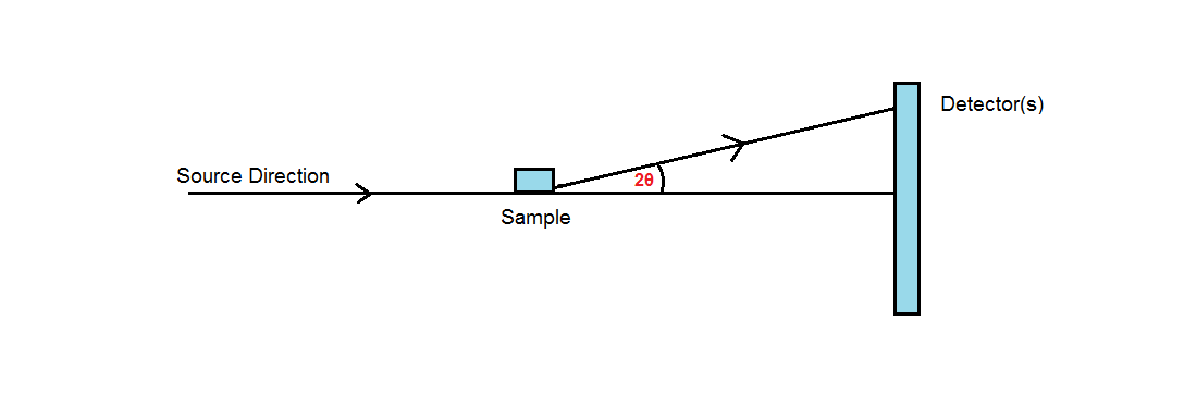
Below we see the typical experimental setup for a Reflectometry instrument. The source direction (Beam vector) is along the horizon. This setup is defined in the Instrument Defintion File and this instrument setup will be attached to any workspaces associated with that instrument. When we pass the IvsLambda workspace to ConvertUnits v1 to produce an IvsQ workspace, ConvertUnits v1 will assume that $2\theta$ is the angle between the Beam vector and the sample-to-detector vector. When we have the typical setup seen below, $2\theta$ will be exactly half the value we wish it to be.

../_images/CurrentExperimentSetupForReflectometry.png

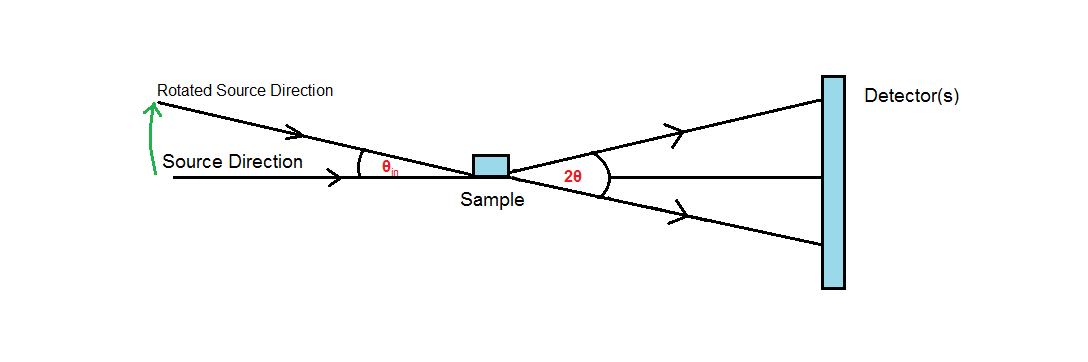
We rotate the position of the Source (and therefore the Beam vector) in the Instrument Defintion associated with the IvsLambda workspace until the condition $\theta_i = \theta_f$ is satisfied. This will achieve the desired result for $2\theta$ (see below for rotated source diagram). After ConvertUnits v1 has produced our IvsQ workspace, we will rotate the position of the source back to its original position so that the experimental setup remains unchanged for other algorithms that may need to manipulate/use it.

../_images/RotatedExperimentSetupForReflectometry.png

Processing Instructions ¶

These enable a grouping pattern on workspace indices to yield only the detectors of interest. It allows usage of the operators ,:+- to specify or exclude specific indices or to add spectra together. See Grouping Pattern from GroupDetectors v2 for further details on their usage.

Usage ¶

Example - Reduce a Run

run = Load(Filename='INTER00013460.nxs')
# Basic reduction with no transmission run
IvsQ, IvsLam, thetaOut = ReflectometryReductionOne(InputWorkspace=run, ThetaIn=0.7, I0MonitorIndex=2, ProcessingInstructions='3:4',
WavelengthMin=1.0, WavelengthMax=17.0,
MonitorBackgroundWavelengthMin=15.0, MonitorBackgroundWavelengthMax=17.0,
MonitorIntegrationWavelengthMin=4.0, MonitorIntegrationWavelengthMax=10.0, Version=1)

print("The first four IvsLam Y values are: [ {:.4e}, {:.4e}, {:.4e}, {:.4e} ]".format(
       IvsLam.readY(0)[0], IvsLam.readY(0)[1], IvsLam.readY(0)[2], IvsLam.readY(0)[3]))
print("The first four IvsQ Y values are: [ {:.4e}, {:.4e}, {:.4e}, {:.4e} ]".format(
       IvsQ.readY(0)[0], IvsQ.readY(0)[1], IvsQ.readY(0)[2], IvsQ.readY(0)[3]))
print("Theta out is the same as theta in: {}".format(thetaOut))

Output:

The first four IvsLam Y values are: [ 0.0000e+00, 0.0000e+00, 7.8118e-07, 1.9346e-06 ]
The first four IvsQ Y values are: [ 1.3845e-03, 1.9717e-03, 2.7579e-03, 4.1467e-03 ]
Theta out is the same as theta in: 0.7

Categories: Algorithms | Reflectometry

Source ¶

C++ source: ReflectometryReductionOne.cpp (last modified: 2017-09-18)

C++ header: ReflectometryReductionOne.h (last modified: 2016-10-19)