Table of Contents
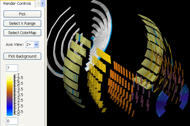
Read a diffraction calibration file (.cal) or an XML grouping file (.xml) and an instrument name, and output a 2D workspace containing on the Y-axis the values of the Group each detector belongs to. This is used to visualise the grouping scheme for powder diffractometers, where a large number of detectors are grouped together. The output 2D workspace can be visualize using the show instrument method.
| Name | Direction | Type | Default | Description |
|---|---|---|---|---|
| InstrumentWorkspace | Input | MatrixWorkspace | Mandatory | A workspace that refers to the instrument of interest. You can use [[LoadEmptyInstrument]] to create such a workspace. |
| GroupingFileName | Input | string | Mandatory | Either as a XML grouping file (see [[GroupDetectors]]) or as a [[CalFile]] (.cal extension). Allowed extensions: [‘.cal’, ‘.xml’] |
| ShowUnselected | Input | string | True | Whether to show detectors that are not in any group. Allowed values: [‘True’, ‘False’] |
| OutputWorkspace | Output | Workspace2D | The name of the output workspace |
 All of the detectors in each group are given the a
value equal to that of the group number. Unselected detectors are given
a value of 0 if ShowUnselected is true.
The instrumentView is the best way to visualize the grouping using the “show Instrument” context menu option on the output workspace.
Note
To run these usage examples please first download the usage data, and add these to your path. In MantidPlot this is done using Manage User Directories.
Example - Read 9 groups for INES instrument:
# Create workspace with INES instrument in it
ws1 = Load("INES_Definition.xml")

# Run algorithm
ws2 = ReadGroupsFromFile( ws1, "INES_example.cal")

# Print the value of selected sprectra. Each corresponds to the group of the corresponding detector.
for i in [0,1,2,3,4,5,6,7,8]:
   print ws2.readY(16*i), ws2.readY(16*i+5), ws2.readY(16*i+10), ws2.readY(16*i+15)
Output:
[ 1.] [ 1.] [ 1.] [ 1.]
[ 2.] [ 2.] [ 2.] [ 2.]
[ 3.] [ 3.] [ 3.] [ 3.]
[ 4.] [ 4.] [ 4.] [ 4.]
[ 5.] [ 5.] [ 5.] [ 5.]
[ 6.] [ 6.] [ 6.] [ 6.]
[ 7.] [ 7.] [ 7.] [ 7.]
[ 8.] [ 8.] [ 8.] [ 8.]
[ 9.] [ 9.] [ 9.] [ 9.]
Categories: Algorithms | Diffraction