SANSWideAngleCorrection v1¶

SANSWideAngleCorrection dialog.

Table of Contents

Summary
Properties
Description
Algorithm Reference Discussion
- Error Propagation
Enabling Wide Angle Correction for Reduction of SANS ISIS
SANS ISIS Reduction
Wide Angle Correction and the SANS Reduction
Comparison with Wide Angle Correction at SNS
References
Usage
Source

Summary ¶

Calculate the Wide Angle correction for SANS transmissions.

Properties ¶

Name	Direction	Type	Default	Description
SampleData	Input	MatrixWorkspace	Mandatory	A workspace cropped to the detector to be reduced (the SAME as the input to [[Q1D]]); used to verify the solid angle. The workspace is not modified, just inspected.
TransmissionData	Input	MatrixWorkspace	Mandatory	The transmission data calculated, referred to as <math>T_0</math> in equations in discussion section
OutputWorkspace	Output	MatrixWorkspace	Mandatory	The transmission corrected SANS data, normalised (divided) by <math>T_0</math>, see discussion section

Algorithm Reference Discussion ¶

Looking at Computing guide for Small Angle Scattering Experiments by Ghosh, Egelhaaf & Rennie, we see that for scattering at larger angles the transmission should be modified due to the longer path length after the scattering event.

The longer path length after scattering will also slightly increase the probability of a second scattering event, but this is not dealt with here.

If our on-axis transmission is $T_0$ through a sample of thickness $d$ , then the transmission at some other thickness $x$ is $\exp(-\mu x)$ where attenuation coefficient $\mu = -\ln( \frac{T_0}{d})$ .

If a neutron scatters at angle $2\theta$ at distance $x$ into the sample, its total transmission is then:

$T^{''} = \exp(-\mu x) \exp( \frac{-\mu(d-x)}{\cos(2\theta)})$

$T^{''}$ should be integrated and averaged between $x = 0$ and $x = d$ .

Hammouda, gives an approximate result for the integral, see page 208 of SANS toolbox:

$T^{'} = \frac{T_0(T_0^A - 1)}{A \ln(T_0)}$

For:

$A = \frac{1}{\cos(2\theta)} - 1$

For example if $T_0 = 0.2$ and $2\theta = 40$ then $T^{'} = 0.158$ , a shift of $~20$ % of the SANS curve. Note that the result is independent of sample thickness.

$T_0$ is a function of neutron wavelength, whilst $A$ is a function of detector pixel location.

The output of this algorithm is:

$OutputWorkspace = \frac{T^\prime}{T_0}$

Error Propagation ¶

The error propagation follows this formula:

$OutputWorkspace_{error} = \frac{T_{0E} ^A - 1}{A\ln(T_0E)}$

Which means, that we do not consider the error in the definition of the $2\theta$ (the parameter A)

Enabling Wide Angle Correction for Reduction of SANS ISIS ¶

To enable the Wide Angle correction use the User File settings:

SAMPLE/PATH/ON

More information on: SANS_User_File_Commands#SAMPLE

SANS ISIS Reduction ¶

The output of SANSWideAngleCorrection is used as WavePixelAdj parameter at Q1D v2.

Wide Angle Correction and the SANS Reduction ¶

The equation for the reduction is (see Q1D v2)

$P_I(Q) = \frac{\sum_{\{i, j, n\} \supset \{I\}} S(i,j,n)}{\sum_{\{i, j, n\} \supset \{I\}}M(n)\eta(n)T(n)\Omega_{i j}F_{i j}}$

But, $T(n)$ is not really $T(n)$ , because of the wide angles, it is now $T(n,theta)$ or $T(n,i,j)$ .

So, we decided to have a new factor that changes this equation to:

$P_I(Q) = \frac{\sum_{\{i, j, n\} \supset \{I\}} S(i,j,n)}{\sum_{\{i, j, n\} \supset \{I\}}M(n)\eta(n)T(n)\Omega_{i j}F_{i j}Corr(i,j,n)}$

Where Corr (Correction factor) in this case will be:

$Corr = \frac{T_0^A - 1}{A \ln(T_0)}$

Which is the OutputWorkspace of SANSWideAngleCorrection.

This parameter enters inside Q1D v2 as WavePixelAdj. But, this is all done for you inside the Reduction Script.

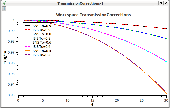
Comparison with Wide Angle Correction at SNS ¶

The transmission correction applied at SNS is described here, and it is applied through the ApplyTransmissionCorrection v1 algorithm. The correction applied there is an approximation for the same equations described here. The picture above compare their results

Note a difference among them is when they are applied. At SNS, the correction is applied before averaging the counters per bin inside Q1D v2 algorithm, while at ISIS, it is used after, inside the Q1D v2 algorithm, for the division of the counters per bin normalized by the transmission counters.

References ¶

Annie Brulet et al. - Improvement of data treatment in small-angle neutron scattering - J. Appl. Cryst. (2007). 40

Ghosh, Egelhaaf & Rennie - Computing guide for Small Angle Scattering Experiments

Usage ¶

Example - Correcting Some Dummy Data

# Create some dummy data, but crop it for quick demonstration purposes.
sample = CreateSimulationWorkspace(Instrument='SANS2D', BinParams=[5,500,100005], UnitX='TOF')
sample = CropWorkspace(sample,StartWorkspaceIndex=0,EndWorkspaceIndex=20)

# Create a dummy transmission workspace.
transmission = CropWorkspace(sample,StartWorkspaceIndex=10,EndWorkspaceIndex=10)
transmission *= 2

corrected_data = SANSWideAngleCorrection(sample, transmission)

print "%f was corrected to %f." % (sample.readY(19)[0], corrected_data.readY(19)[0])

Output:

1.000000 was corrected to 1.004997.

Categories: Algorithms | CorrectionFunctions | TransmissionCorrections

Source ¶

Python: SANSWideAngleCorrection.py