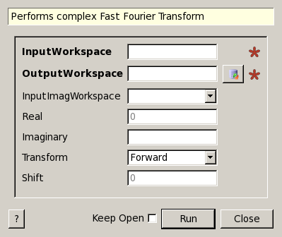
FFT dialog.
Table of Contents
| Name | Direction | Type | Default | Description |
|---|---|---|---|---|
| InputWorkspace | Input | MatrixWorkspace | Mandatory | The name of the input workspace. |
| OutputWorkspace | Output | MatrixWorkspace | Mandatory | The name of the output workspace. |
| InputImagWorkspace | Input | MatrixWorkspace | The name of the input workspace for the imaginary part. Leave blank if same as InputWorkspace | |
| Real | Input | number | 0 | Spectrum number to use as real part for transform |
| Imaginary | Input | number | Optional | Spectrum number to use as imaginary part for transform |
| Transform | Input | string | Forward | Direction of the transform: forward or backward. Allowed values: [‘Forward’, ‘Backward’] |
| Shift | Input | number | 0 | Apply an extra phase equal to this quantity times 2*pi to the transform |
The FFT algorithm performs discrete Fourier transform of complex data using the Fast Fourier Transform algorithm. It uses the GSL Fourier transform functions to do the calculations. Due to the nature of the fast fourier transform the input spectra must have linear x axes. If the imaginary part is not set the data is considered real. The “Transform” property defines the direction of the transform: direct (“Forward”) or inverse (“Backward”).
Note that the input data is shifted before the transform along the x
axis to place the origin in the middle of the x-value range. It means
that for the data defined on an interval [A,B] the output
 must be multiplied by
  ,
where
,
where 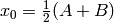 ,
,  is the frequency.
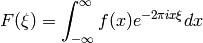
The Fourier transform of a complex function  is defined by
equation:
is defined by
equation:
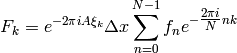
For discrete data with equally spaced  and only non-zero on
an interval
and only non-zero on
an interval ![[A,B]](../_images/math/8fedf99daa76b293f2e09845b6316f98e38036c7.png) the integral can be approximated by a sum:
the integral can be approximated by a sum:
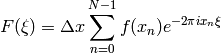
Here  is the bin width,
  . If we
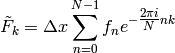
are looking for values of the transformed function
. If we
are looking for values of the transformed function  at discrete
frequencies
at discrete
frequencies  with
with
the equation can be rewritten:
Here  and
and  . The formula
is the Discrete Fourier Transform (DFT) and can be efficiently evaluated
using the Fast Fourier Transform algorithm. The DFT formula calculates
the Fourier transform of data on the interval ![[0,L]](../_images/math/50922c76bfd9c9e64038ae352f70b736108988f1.png) . It should
be noted that it is periodic in
. It should
be noted that it is periodic in  with period
  . If we
also assume that
. If we
also assume that  is also periodic with period the
DFT can be used to transform data on the interval
is also periodic with period the
DFT can be used to transform data on the interval ![[-L/2,L/2]](../_images/math/8e7d252c63ee5f64495f507b0a825b2b1ceb9b4a.png) . To
do this we swap the two halves of the data array . If we
denote the modified array as
. To
do this we swap the two halves of the data array . If we
denote the modified array as  , its transform will be
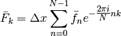
The Mantid FFT algorithm returns the complex array  as
Y values of two spectra in the output workspace, one for the real and
the other for the imaginary part of the transform. The X values are set
to the transform frequencies and have the range approximately equal to
as
Y values of two spectra in the output workspace, one for the real and
the other for the imaginary part of the transform. The X values are set
to the transform frequencies and have the range approximately equal to
![[-N/L,N/L]](../_images/math/256515c3fccc96368ac7ad3327b2f91193380f41.png) . The actual limits depend sllightly on whether
is even or odd and whether the input spectra are histograms or
point data. The variations are of the order of
. The actual limits depend sllightly on whether
is even or odd and whether the input spectra are histograms or
point data. The variations are of the order of  . The
zero frequency is always in the bin with index
. The
zero frequency is always in the bin with index 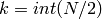 .
.
In this example the input data were calculated using function
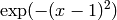 in the range [-5,5].
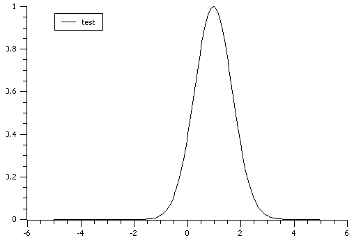
Gaussian
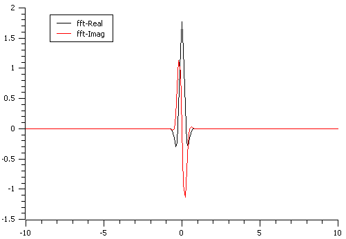
FFT of a Gaussian
Because the  is in the middle of the data array the transform
shown is the exact DFT of the input data.
is in the middle of the data array the transform
shown is the exact DFT of the input data.
In this example the input data were calculated using function
 in the range [-6,4].
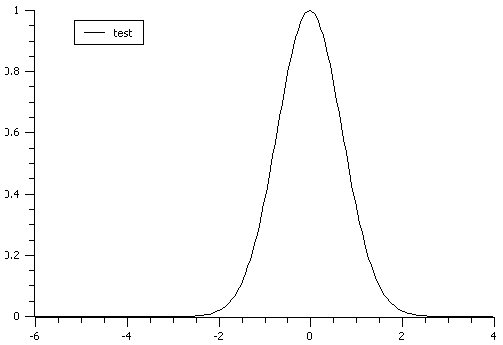
Gaussian
FFT of a Gaussian
Because the is not in the middle of the data array the
transform shown includes a shifting factor of  .
To remove it the output must be mulitplied by
.
To remove it the output must be mulitplied by  .
The corrected transform will be:
.
The corrected transform will be:
FFT of a Gaussian
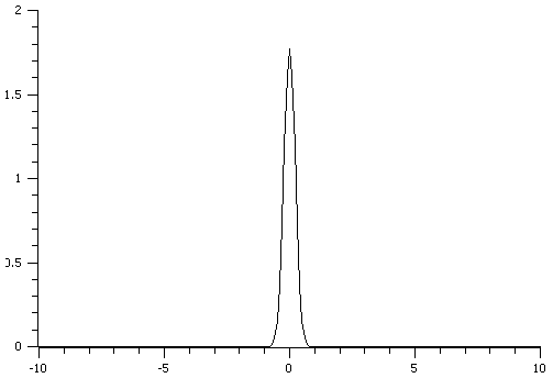
It should be noted that in a case like this, i.e. when the input is a
real positive even function, the correction can be done by finding the
transform’s modulus 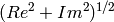 . The output workspace
includes the modulus of the transform.
. The output workspace
includes the modulus of the transform.
The output workspace for a direct (“Forward”) transform contains either
three or six spectra, depending on whether the input function is complex
or purely real. If the input function has an imaginary part, the
transform is written to three spectra with indexes 0, 1, and 2. Indexes
0 and 1 are the real and imaginary parts, while index 2 contains the
modulus  . If the input function does not contain
an spectrum for the imaginary part (purely real function), the actual
transform is written to spectra with indexes 3 and 4 which are the real
and imaginary parts, respectively. The last spectrum (index 5) has the
modulus of the transform. The spectra from 0 to 2 repeat these results
for positive frequencies only.
. If the input function does not contain
an spectrum for the imaginary part (purely real function), the actual
transform is written to spectra with indexes 3 and 4 which are the real
and imaginary parts, respectively. The last spectrum (index 5) has the
modulus of the transform. The spectra from 0 to 2 repeat these results
for positive frequencies only.
Output for the case of input function containing imaginary part:
| Workspace index | Description |
|---|---|
| 0 | Complete real part |
| 1 | Complete imaginary part |
| 2 | Complete transform modulus |
Output for the case of input function containing no imaginary part:
| Workspace index | Description |
|---|---|
| 0 | Real part, positive frequencies |
| 1 | Imaginary part, positive frequencies |
| 2 | Modulus, positive frequencies |
| 3 | Complete real part |
| 4 | Complete imaginary part |
| 5 | Complete transform modulus |
The output workspace for an inverse (“Backward”) transform has 3 spectra for the real (0), imaginary (1) parts, and the modulus (2).
| Workspace index | Description |
|---|---|
| 0 | Real part |
| 1 | Imaginary part |
| 2 | Modulus |
Example: Applying FFT algorithm
#Create Sample Workspace
ws = CreateSampleWorkspace(WorkspaceType = 'Event', NumBanks = 1, Function = 'Exp Decay', BankPixelWidth = 1, NumEvents = 100)

#apply the FFT algorithm
outworkspace = FFT(InputWorkspace = ws, Transform = 'Backward')

#print statements
print "DataX(0)[0] equals DataX(0)[100]? : " + str((round(abs(outworkspace.dataX(0)[0]), 3)) == (round(outworkspace.dataX(0)[100], 3)))
print "DataX(0)[10] equals DataX(0)[90]? : " + str((round(abs(outworkspace.dataX(0)[10]), 3)) == (round(outworkspace.dataX(0)[90], 3)))
print "DataX((0)[50] equals 0? : " + str((round(abs(outworkspace.dataX(0)[50]), 3)) == 0)
print "DataY(0)[40] equals DataY(0)[60]? : " + str((round(abs(outworkspace.dataY(0)[40]), 5)) == (round(outworkspace.dataY(0)[60], 5)))
Output:
DataX(0)[0] equals DataX(0)[100]? : True
DataX(0)[10] equals DataX(0)[90]? : True
DataX((0)[50] equals 0? : True
DataY(0)[40] equals DataY(0)[60]? : True
Categories: Algorithms | Arithmetic\FFT