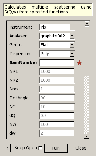
MuscatFunc dialog.
Table of Contents
| Name | Direction | Type | Default | Description |
|---|---|---|---|---|
| Instrument | Input | string | iris | Instrument. Allowed values: [‘irs’, ‘iris’, ‘osi’, ‘osiris’] |
| Analyser | Input | string | graphite002 | Allowed values: [‘graphite002’, ‘graphite004’] |
| Geom | Input | string | Flat | Allowed values: [‘Flat’, ‘Cyl’] |
| Dispersion | Input | string | Poly | Allowed values: [‘Poly’, ‘CE’, ‘SS’] |
| SamNumber | Input | string | Mandatory | Sample data run number |
| NR1 | Input | number | 1000 | MonteCarlo neutrons NR1. Default=1000 |
| NR2 | Input | number | 1000 | MonteCarlo neutrons NR2. Default=1000 |
| Nms | Input | number | 1 | Number of scatterings. Default=1 |
| DetAngle | Input | number | 90 | Detector angle. Default=90.0 |
| NQ | Input | number | 10 | Q-w grid: number of Q values. Default=10 |
| dQ | Input | number | 0.2 | Q-w grid: Q increment. Default=0.2 |
| NW | Input | number | 100 | Q-w grid: number of w values. Default=100 |
| dW | Input | number | 2 | Q-w grid: w increment (microeV). Default=2.0 |
| Coeff1 | Input | number | 0 | Coefficient 1. Default=0.0 |
| Coeff2 | Input | number | 0 | Coefficient 2. Default=0.0 |
| Coeff3 | Input | number | 50 | Coefficient 3. Default=50.0 |
| Coeff4 | Input | number | 0 | Coefficient 4. Default=0.0 |
| Coeff5 | Input | number | 0 | Coefficient 5. Default=0.0 |
| Thick | Input | string | Mandatory | Sample thickness |
| Width | Input | string | Mandatory | Sample width |
| Height | Input | number | 3 | Sample height. Default=3.0 |
| Density | Input | number | 0.1 | Sample density. Default=0.1 |
| SigScat | Input | number | 5 | Scattering cross-section. Default=5.0 |
| SigAbs | Input | number | 0.1 | Absorption cross-section. Default=0.1 |
| Temperature | Input | number | 300 | Sample temperature (K). Default=300.0 |
| Plot | Input | string | None | Allowed values: [‘None’, ‘Totals’, ‘Scat1’, ‘All’] |
| Verbose | Input | boolean | True | Switch Verbose Off/On |
| Save | Input | boolean | False | Switch Save result to nxs file Off/On |
Calculates Multiple Scattering based on the Monte Carlo program MINUS.
It calculates  from specified functions (such as those
used in JumpFit) and supports both Flat and Cylindrical geometries. More
information on the multiple scattering can be procedure can be found in
the modes
manual.
from specified functions (such as those
used in JumpFit) and supports both Flat and Cylindrical geometries. More
information on the multiple scattering can be procedure can be found in
the modes
manual.
Example - a basic example using MuscatFunc.
def createSampleWorkspace(name, random=False):
        """ Creates a sample workspace with a single lorentzian that looks like IRIS data"""
        import os
        function = "name=Lorentzian,Amplitude=8,PeakCentre=5,FWHM=0.7"
        ws = CreateSampleWorkspace("Histogram", Function="User Defined", UserDefinedFunction=function, XUnit="DeltaE", Random=True, XMin=0, XMax=10, BinWidth=0.01)
        ws = CropWorkspace(ws, StartWorkspaceIndex=0, EndWorkspaceIndex=9)
        ws = ScaleX(ws, -5, "Add")
        ws = ScaleX(ws, 0.1, "Multiply")

        #load instrument and instrument parameters
        LoadInstrument(ws, InstrumentName='IRIS', RewriteSpectraMap=True)
        path = os.path.join(config['instrumentDefinition.directory'], 'IRIS_graphite_002_Parameters.xml')
        LoadParameterFile(ws, Filename=path)
        ws = RenameWorkspace(ws, OutputWorkspace=name)
        return ws


ws = createSampleWorkspace("irs26173_graphite002_red", random=True)
SaveNexus(ws, "irs26173_graphite002_red.nxs")

MuscatFunc(SamNumber='26173', Thick='0.5', Width='0.5', Instrument='irs')
Categories: Algorithms | Workflow\MIDAS
Python: MuscatFunc.py