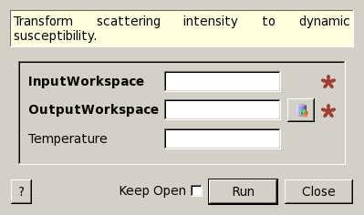
ApplyDetailedBalance v1¶

ApplyDetailedBalance dialog.

Table of Contents

Summary
Properties
Description
Usage
Source

Summary ¶

Transform scattering intensity to dynamic susceptibility.

Properties ¶

Name	Direction	Type	Default	Description
InputWorkspace	Input	MatrixWorkspace	Mandatory	An input workspace.
OutputWorkspace	Output	MatrixWorkspace	Mandatory	An output workspace.
Temperature	Input	string		SampleLog variable name that contains the temperature, or a number

Description ¶

The fluctuation dissipation theorem [1,2] relates the dynamic susceptibility to the scattering function

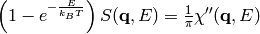
$\left(1-e^{-\frac{E}{k_B T}}\right) S(\mathbf{q}, E) = \frac{1}{\pi} \chi'' (\mathbf{q}, E)$

where $E$ is the energy transfer to the system. The algorithm assumes that the y axis of the input workspace contains the scattering function $S$ . The y axis of the output workspace will contain the dynamic susceptibility. The temperature is extracted from a log attached to the workspace, as the mean value. Alternatively, the temperature can be directly specified. The algorithm will fail if neither option is valid.

[1] S. W. Lovesey - Theory of Neutron Scattering from Condensed Matter, vol 1

[2] I. A. Zaliznyak and S. H. Lee - Magnetic Neutron Scattering in “Modern techniques for characterizing magnetic materials”

Usage ¶

Example - Run Applied Detailed Balance

ws = CreateWorkspace(DataX='-5,-4,-3,-2,-1,0,1,2,3,4,5',DataY='2,2,2,2,2,2,2,2,2,2',DataE='1,1,1,1,1,1,1,1,1,1',UnitX='DeltaE')
ows = ApplyDetailedBalance(InputWorkspace='ws',OutputWorkspace='ows',Temperature='100')

print "The Y values in the Output Workspace are"
print str(ows.readY(0)[0:5])
print str(ows.readY(0)[5:10])

Output:

The Y values in the Output Workspace are
[-4.30861792 -3.14812682 -2.11478496 -1.19466121 -0.37535083]
[ 0.35419179  1.00380206  1.58223777  2.09729717  2.55592407]

Categories: Algorithms | Inelastic\Corrections