BayesQuasi dialog.
Table of Contents
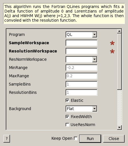
This algorithm runs the Fortran QLines programs which fits a Delta function of amplitude 0 and Lorentzians of amplitude A(j) and HWHM W(j) where j=1,2,3. The whole function is then convoled with the resolution function.
| Name | Direction | Type | Default | Description |
|---|---|---|---|---|
| Program | Input | string | QL | The type of program to run (either QL or QSe). Allowed values: [‘QL’, ‘QSe’] |
| SampleWorkspace | Input | MatrixWorkspace | Mandatory | Name of the Sample input Workspace |
| ResolutionWorkspace | Input | MatrixWorkspace | Mandatory | Name of the resolution input Workspace |
| ResNormWorkspace | Input | WorkspaceGroup | Name of the ResNorm input Workspace | |
| MinRange | Input | number | -0.2 | The start of the fit range. Default=-0.2 |
| MaxRange | Input | number | 0.2 | The end of the fit range. Default=0.2 |
| SampleBins | Input | number | 1 | The number of sample bins |
| ResolutionBins | Input | number | 1 | The number of resolution bins |
| Elastic | Input | boolean | True | Fit option for using the elastic peak |
| Background | Input | string | Flat | Fit option for the type of background. Allowed values: [‘Sloping’, ‘Flat’, ‘Zero’] |
| FixedWidth | Input | boolean | True | Fit option for using FixedWidth |
| UseResNorm | Input | boolean | False | fit option for using ResNorm |
| WidthFile | Input | string | The name of the fixedWidth file | |
| Loop | Input | boolean | True | Switch Sequential fit On/Off |
| Plot | Input | string | Plot options | |
| Save | Input | boolean | False | Switch Save result to nxs file Off/On |
| OutputWorkspaceFit | Output | WorkspaceGroup | Mandatory | The name of the fit output workspaces |
| OutputWorkspaceResult | Output | MatrixWorkspace | Mandatory | The name of the result output workspaces |
| OutputWorkspaceProb | Output | MatrixWorkspace | The name of the probability output workspaces |
This algorith can only be run on windows due to f2py support and the underlying fortran code
The model that is being fitted is that of a delta-function (elastic component) of amplitude A(0) and Lorentzians of amplitude A(j) and HWHM W(j) where j=1,2,3. The whole function is then convolved with the resolution function. The -function and Lorentzians are intrinsically normalised to unity so that the amplitudes represent their integrated areas.
For a Lorentzian, the Fourier transform does the conversion:
![1/(x^{2}+\delta^{2}) \Leftrightarrow exp[-2\pi(\delta k)]](../_images/math/8cfe2d45d1b9de22f5e1b9f503b4a0353b75086f.png) .
If x is identified with energy E and
.
If x is identified with energy E and  where t is time then:
![1/[E^{2}+(\hbar / \tau)^{2}] \Leftrightarrow exp[-t/\tau]](../_images/math/141dc68b232294ff4235145938fd415e95e2788d.png) and
and  is identified with
  The program estimates the quasielastic components of each of the groups of spectra and requires the resolution
file and optionally the normalisation file created by ResNorm.
The program estimates the quasielastic components of each of the groups of spectra and requires the resolution
file and optionally the normalisation file created by ResNorm.
For a Stretched Exponential, the choice of several Lorentzians is replaced with a single function with the shape :
![\psi\beta(x) \Leftrightarrow exp[-2\pi(\sigma k)\beta]](../_images/math/364a3414ec4a8c1e73d8b4a1f4bfed39ae740039.png) . This, in the energy to time FT transformation,
is
. This, in the energy to time FT transformation,
is ![\psi\beta(E) \Leftrightarrow exp[-(t/\tau)\beta]](../_images/math/a107edd8fafd9951836b41fc46f0bfdd89b363db.png) . So is identified with
. So is identified with  .
The model that is fitted is that of an elastic component and the stretched exponential and the program gives the best estimate
for the
.
The model that is fitted is that of an elastic component and the stretched exponential and the program gives the best estimate
for the  parameter and the width for each group of spectra.
Example - BayesQuasi
# Check OS support for F2Py
from IndirectImport import is_supported_f2py_platform
if is_supported_f2py_platform():
    # Load in test data
    sampleWs = Load('irs26176_graphite002_red.nxs')
    resWs = Load('irs26173_graphite002_red.nxs')

    # Run BayesQuasi algorithm
    fit_ws, result_ws, prob_ws = BayesQuasi(Program='QL', SampleWorkspace=sampleWs, ResolutionWorkspace=resWs,
                                        MinRange=-0.547607, MaxRange=0.543216, SampleBins=1, ResolutionBins=1,
                                        Elastic=False, Background='Sloping', FixedWidth=False, UseResNorm=False,
                                        WidthFile='', Loop=True, Save=False, Plot='None')
Categories: Algorithms | Workflow\MIDAS
Python: BayesQuasi.py