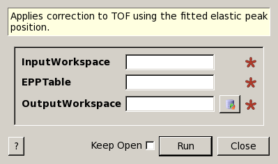
CorrectTOF dialog.
Table of Contents
| Name | Direction | Type | Default | Description |
|---|---|---|---|---|
| InputWorkspace | Input | MatrixWorkspace | Mandatory | Input workspace. |
| EPPTable | Input | TableWorkspace | Mandatory | Input EPP table. May be produced by FindEPP algorithm. |
| OutputWorkspace | Output | MatrixWorkspace | Mandatory | Name of the workspace that will contain the results |
This algorithm applies to the time-of-flight correction which considers the specified elastic peak position. The new X-axis data  are calculated as
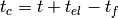
where  is the time-of-flight in the input workspace,
  is the theoretical elastic time-of-flight, calculated from the neutron wavelength and sample-detector distance,
  is the time-of-flight from sample to detector, corresponding to the elastic peak position specified in the EPPTable.
Note
The input EPPTable can be produced using the FindEPP v1 algorithm.
If position of the elastic peak is  for a particular detector, this detector will be masked in the output workspace and warning will be produced. No correction is applied in this case.
Example 1: Apply correction to a sample workspace.
# create workspace with appropriate sample logs
ws = CreateSampleWorkspace(Function="User Defined", UserDefinedFunction="name=LinearBackground, \
                           A0=0.3;name=Gaussian, PeakCentre=8123.34, Height=5, Sigma=75", NumBanks=1,
                           BankPixelWidth=1, XMin=6005.25, XMax=9995.75, BinWidth=10.5,
                           BankDistanceFromSample=4.0, OutputWorkspace="ws",SourceDistanceFromSample=1.4)

lognames = "wavelength,TOF1"
logvalues = "6.0,2123.34"
AddSampleLogMultiple(ws, lognames, logvalues)

# create the EPP table
table = CreateEmptyTableWorkspace(OutputWorkspace="epptable")
table.addColumn(type="double", name="PeakCentre")
table_row = {'PeakCentre': 8128.59}
for i in range(ws.getNumberHistograms()):
    table.addRow(table_row)

# apply correction
wscorr = CorrectTOF(ws, table)

print "Correction term dt = t_el - t_table = ", round(8190.02 - 8128.59, 2)
difference = wscorr.readX(0) - ws.readX(0)
print "Difference between input and corrected workspaces: ", round(difference[10],2)
Output:
Correction term dt = t_el - t_table =  61.43
Difference between input and corrected workspaces:  61.43
Example 2: Apply correction to the TOFTOF data.
import numpy

# load TOFTOF data
ws_tof = LoadMLZ(Filename='TOFTOFTestdata.nxs')

# find elastic peak positions
epptable = FindEPP(ws_tof)

# apply TOF correction
ws_tof_corr = CorrectTOF(ws_tof, epptable)

# apply units conversion to the corrected workspace
ws_dE = ConvertUnits(ws_tof_corr, Target='DeltaE', EMode='Direct', EFixed=2.27)
ConvertToDistribution(ws_dE)

print "5 X values of raw data: ", numpy.round(ws_tof.readX(200)[580:585],2)
print "5 X values corrected data: ", numpy.round(ws_tof_corr.readX(200)[580:585],2)
print "5 X values after units conversion: ", numpy.round(ws_dE.readX(200)[580:585], 2)
Output:
5 X values of raw data:  [ 8218.59  8229.09  8239.59  8250.09  8260.59]
5 X values corrected data:  [ 8218.61  8229.11  8239.61  8250.11  8260.61]
5 X values after units conversion:  [ 0.02  0.03  0.03  0.04  0.05]
Categories: Algorithms | Workflow\MLZ\TOFTOF | Transforms\Axes
Python: CorrectTOF.py