MaxEnt v1¶

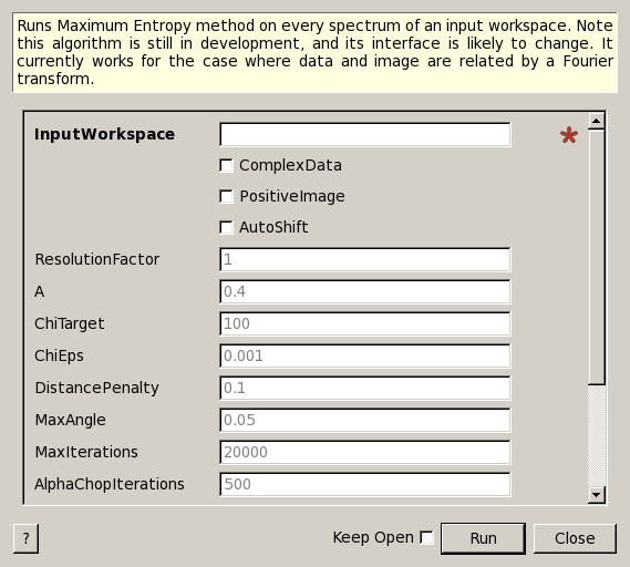
MaxEnt dialog.

Table of Contents

Summary
Properties
Description
Output Workspaces
Usage
Positive Images
Increasing the number of points in the image
References
Source

Summary ¶

Runs Maximum Entropy method on every spectrum of an input workspace. Note this algorithm is still in development, and its interface is likely to change. It currently works for the case where data and image are related by a Fourier transform.

Properties ¶

Name	Direction	Type	Default	Description
InputWorkspace	Input	MatrixWorkspace	Mandatory	An input workspace.
ComplexData	Input	boolean	False	Whether or not the input data are complex. If true, the input workspace is expected to have an even number of histograms.
PositiveImage	Input	boolean	False	If true, the reconstructed image must be positive. It can take negative values otherwise
AutoShift	Input	boolean	False	Automatically calculate and apply phase shift. Zero on the X axis is assumed to be in the first bin. If it is not, setting this property will automatically correct for this.
ResolutionFactor	Input	m	1	An integer number indicating the factor by which the number of points will be increased in the image and reconstructed data
A	Input	number	0.4	A maximum entropy constant
ChiTarget	Input	number	100	Target value of Chi-square
ChiEps	Input	number	0.001	Required precision for Chi-square
DistancePenalty	Input	number	0.1	Distance penalty applied to the current image
MaxAngle	Input	number	0.05	Maximum degree of non-parallelism between S and C
MaxIterations	Input	m	20000	Maximum number of iterations
AlphaChopIterations	Input	m	500	Maximum number of iterations in alpha chop
EvolChi	Output	MatrixWorkspace	Mandatory	Output workspace containing the evolution of Chi-sq
EvolAngle	Output	MatrixWorkspace	Mandatory	Output workspace containing the evolution of non-paralellism between S and C
ReconstructedImage	Output	MatrixWorkspace	Mandatory	The output workspace containing the reconstructed image.
ReconstructedData	Output	MatrixWorkspace	Mandatory	The output workspace containing the reconstructed data.

Description ¶

The maximum entropy method (MEM) is used as a signal processing technique for reconstructing images from noisy data. It selects a single image from the many images which fit the data with the same value of the statistic, $\chi^2$ . The maximum entropy method selects from this feasible set of images, the one which has minimum information (maximum entropy). More specifically, the algorithm maximizes the entropy $S\left(x\right)$ subject to the constraint:

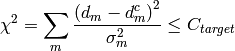
$\chi^2 = \sum_m \frac{\left(d_m - d_m^c\right)^2}{\sigma_m^2} \leq C_{target}$

where $d_m$ are the experimental data, $\sigma_m$ the associated errors, and $d_m^c$ the calculated or reconstructed data. The image is the set of numbers 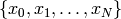$\{x_0, x_1, \dots, x_N\}$ which relates to the measured data as:

$d_m = \sum_j M_{mj} x_j$

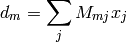
where the measurement kernel matrix $\mathbf{M}$ represents a Fourier transform, $M_{mj} = \exp\left(-ik_mj\right)$ . At present, nothing is assumed about $x_j$ : it can be either positive or negative and real or complex, and the entropy is defined as

$S = \sum_j \left(x_j/A\right) \sinh^{-1} \left(x_j/A\right)$

where $A$ is a constant. The sensitive of the reconstructed image to reconstructed image will vary depending on the data. In general a smaller value would preduce a sharper image. See section 4.7 in Ref. [1] for recommended strategy to selected $A$ .

The implementation used to find the solution where the entropy is maximized subject to the constraint in $\chi^2$ follows the approach by Skilling & Bryan [2], which is an algorithm that is not explicitly using Lagrange multiplier. Instead, they construct a subspace from a set of search directions to approach the maximum entropy solution. Initially, the image $x$ is set to the flat background $A$ and the search directions are constructed using the gradients of $S$ and $\chi^2$ :

$\mathbf{e}_1 = f\left(\nabla S\right)$

$\mathbf{e}_2 = f\left(\nabla \chi^2\right)$

where $f\left(\nabla S\right)$ stands for a componentwise multiplication. The algorithm next uses a quadratic approximation to determine the increment $\delta \mathbf{x}$ that moves the image one step closer to the solution:

$\mathbf{x} = \mathbf{x} + \delta \mathbf{x}$

Output Workspaces ¶

There are four output workspaces: ReconstructedImage and ReconstructedData contain the image and calculated data respectively, and EvolChi and EvolAngle record the algorithm’s evolution. ReconstructedData can be used to check that the calculated data approaches the experimental, measured data, and ReconstructedImage corresponds to its Fourier transform. If the input data are real they contain twice the original number of spectra, as the Fourier transform will be a complex signal in general. The real and imaginary parts are organized as follows (see Table 1): assuming your input workspace has $M$ spectra, the real part of the reconstructed spectrum $s$ corresponds to spectrum $s$ in the output workspaces ReconstructedImage and ReconstructedData, while the imaginary part can be found in spectrum $s+M$ .

When the input data are complex, the input workspace is expected to have $2M$ spectra, where real and imaginary parts of input $s$ , are arranged in spectra $(s, s+M)$ respectively. In other words, ReconstructedData and ReconstructedImage will contain $2M$ spectra, where spectra $(s, s+M)$ correspond to the real and imaginary parts reconstructed from the input signal at $(s, s+M)$ in the input workspace (see Table 2 below).

The workspaces EvolChi and EvolAngle record the evolution of $\chi^2$ and the angle (or non-parallelism) between $\nabla S$ and $\nabla \chi^2$ . Note that the algorithm runs until a solution is found, and that an image is considered to be a true maximum entropy solution when the following two conditions are met simultaneously:

$\chi^2_{Target} - \chi^2 < \epsilon_1, \qquad \frac{1}{2} \left| \frac{\nabla S}{\left|\nabla S\right|} - \frac{\nabla \chi^2}{\left|\nabla \chi^2\right|} \right| < \epsilon_2$

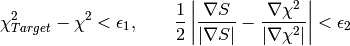
While one of these conditions is not satisfied the algorithm keeps running until it reaches the maximum number of iterations. When the maximum number of iterations is reached, the last reconstructed image and its corresponding calculated data are returned, even if they do not correspond to a true maximum entropy solution satisfying the conditions above. In this way, the user can check by inspecting the output workspaces whether the algorithm was evolving towards the correct solution or not. On the other hand, the user must always check the validity of the solution by inspecting EvolChi and EvolAngle, whose values will be set to zero once the true maximum entropy solution is found.

Table 1. Output workspaces for the case of real data (M histograms and N bins in the input workspace)
Workspace	Number of histograms	Number of bins	Description
EvolChi	M	MaxIterations	Evolution of $\chi^2$ until the solution is found. Then all values are set to zero.
EvolAngle	M	MaxIterations	Evolution of the angle between $\nabla S$ and $\nabla \chi^2$ , until the solution is found. Then all values are set to zero.
ReconstructedImage	2M	N	For spectrum $s$ in the input workspace, the reconstructed image is stored in spectra $s$ (real part) and $s+M$ (imaginary part)
ReconstructedData	2M	N	For spectrum $s$ in the input workspace, the reconstructed data are stored in spectrum $s$ (real part) and $s+M$ (imaginary part). Note that although the input is real, the imaginary part is recorded for debugging purposes, it should be zero for all data points.

Table 2. Output workspaces for the case of complex input (2M histograms and N bins in the input workspace. Real and imaginary parts must be consecutive)
Workspace	Number of histograms	Number of bins	Description
EvolChi	M	MaxIterations	Evolution of $\chi^2$ until the solution is found. Then all values are set to zero.
EvolAngle	M	MaxIterations	Evolution of the angle between $\nabla S$ and $\nabla \chi^2$ , until the solution is found. Then all values are set to zero.
ReconstructedImage	2M	$N$	For spectrum $(s, s+M)$ in the input workspace, the reconstructed image is stored in spectra $s$ (real part) and $s+M$ (imaginary part)
ReconstructedData	2M	$N$	For spectrum $(s, s+M)$ in the input workspace, the reconstructed data are stored in spectra $s$ (real part) and $s+M$ (imaginary part)

Usage ¶

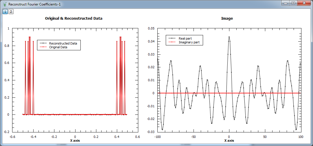
Example - Reconstruct Fourier coefficients

In the example below, a workspace containing five Fourier coefficients is created and used as input to MaxEnt v1. In the figure we show the original and reconstructed data (left), and the reconstructed image, i.e. Fourier transform (right).

# Create an empty workspace
X = []
Y = []
E = []
N = 200
for i in range(0,N):
    x = ((i-N/2) *1./N)
    X.append(x)
    Y.append(0)
    E.append(0.001)

# Fill in five Fourier coefficients
# The input signal must be symmetric
Y[5] = Y[195] = 0.85
Y[10] = Y[190] = 0.85
Y[20] = Y[180] = 0.85
Y[12] = Y[188] = 0.90
Y[14] = Y[186] = 0.90
CreateWorkspace(OutputWorkspace='inputws',DataX=X,DataY=Y,DataE=E,NSpec=1)
evolChi, evolAngle, image, data = MaxEnt(InputWorkspace='inputws', chiTarget=N, A=0.0001)

print "First  reconstructed coefficient: %.3f" % data.readY(0)[5]
print "Second reconstructed coefficient: %.3f" % data.readY(0)[10]
print "Third  reconstructed coefficient: %.3f" % data.readY(0)[20]
print "Fourth reconstructed coefficient: %.3f" % data.readY(0)[12]
print "Fifth  reconstructed coefficient: %.3f" % data.readY(0)[14]

Output:

First  reconstructed coefficient: 0.849
Second reconstructed coefficient: 0.847
Third  reconstructed coefficient: 0.848
Fourth reconstructed coefficient: 0.901
Fifth  reconstructed coefficient: 0.899

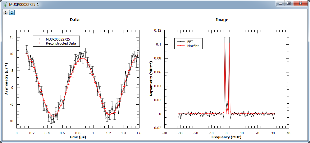
../_images/MaxEntFourierCoefficients.png

Example - Reconstruct a real muon dataset

In this example, MaxEnt v1 is run on a pre-analyzed muon dataset. The corresponding figure shows the original and reconstructed data (left), and the real part of the image obtained with MaxEnt v1 and FFT v1 (right).

Load(Filename=r'MUSR00022725.nxs', OutputWorkspace='MUSR00022725')
CropWorkspace(InputWorkspace='MUSR00022725', OutputWorkspace='MUSR00022725', XMin=0.11, XMax=1.6, EndWorkspaceIndex=0)
RemoveExpDecay(InputWorkspace='MUSR00022725', OutputWorkspace='MUSR00022725')
Rebin(InputWorkspace='MUSR00022725', OutputWorkspace='MUSR00022725', Params='0.016')
evolChi, evolAngle, image, data = MaxEnt(InputWorkspace='MUSR00022725', A=0.005, ChiTarget=90)
# Compare MaxEnt to FFT
imageFFT = FFT(InputWorkspace='MUSR00022725')

print "Image at %.3f: %.3f" % (image.readX(0)[44], image.readY(0)[44])
print "Image at %.3f: %.3f" % (image.readX(0)[46], image.readY(0)[46])
print "Image at %.3f: %.3f" % (image.readX(0)[48], image.readY(0)[48])

Output:

Image at -1.359: 0.102
Image at 0.000: 0.010
Image at 1.359: 0.102

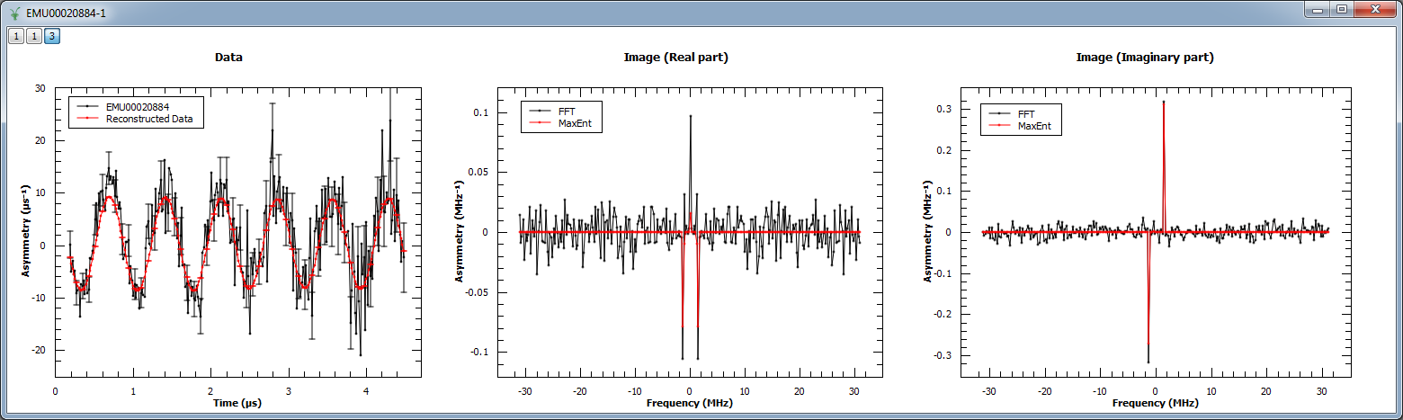
Next, MaxEnt v1 is run on a different muon dataset. The figure shows the original and reconstructed data (left), the real part of the image (middle) and its imaginary part (right).

Load(Filename=r'EMU00020884.nxs', OutputWorkspace='EMU00020884')
CropWorkspace(InputWorkspace='EMU00020884', OutputWorkspace='EMU00020884', XMin=0.17, XMax=4.5, EndWorkspaceIndex=0)
RemoveExpDecay(InputWorkspace='EMU00020884', OutputWorkspace='EMU00020884')
Rebin(InputWorkspace='EMU00020884', OutputWorkspace='EMU00020884', Params='0.016')
evolChi, evolAngle, image, data = MaxEnt(InputWorkspace='EMU00020884', A=0.0001, ChiTarget=300, MaxIterations=2500)
# Compare MaxEnt to FFT
imageFFT = FFT(InputWorkspace='EMU00020884')

print "Image (real part) at %.3f: %.3f" % (image.readX(0)[129], image.readY(0)[129])
print "Image (real part) at  %.3f:  %.3f" % (image.readX(0)[135], image.readY(0)[135])
print "Image (real part) at  %.3f: %.3f" % (image.readX(0)[141], image.readY(0)[141])
print "Image (imaginary part) at %.3f: %.3f" % (image.readX(0)[129], image.readY(0)[129])
print "Image (imaginary part) at  %.3f:  %.3f" % (image.readX(0)[135], image.readY(0)[135])
print "Image (imaginary part) at  %.3f: %.3f" % (image.readX(0)[141], image.readY(0)[141])

Output:

Image (real part) at -1.389: -0.079
Image (real part) at  0.000:  0.015
Image (real part) at  1.389: -0.079
Image (imaginary part) at -1.389: -0.079
Image (imaginary part) at  0.000:  0.015
Image (imaginary part) at  1.389: -0.079

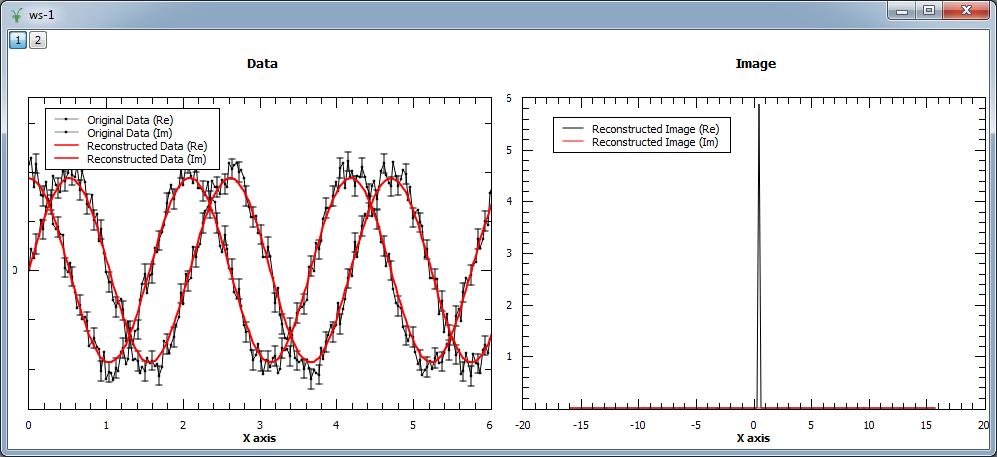
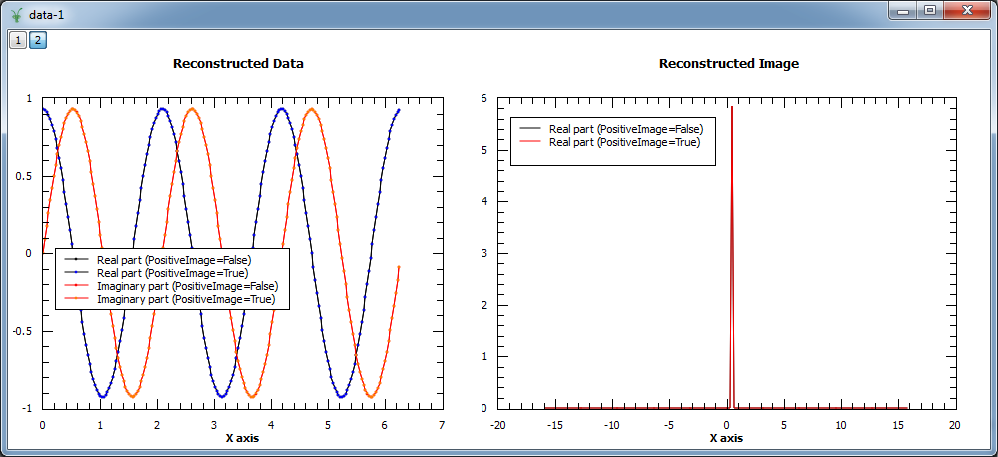
Finally, we show an example where a complex signal is analyzed. In this case, the input workspace contains two spectra corresponding to the real and imaginary part of the same signal. The figure shows the original and reconstructed data (left), and the reconstructed image (right).

from math import pi, sin, cos
from random import random, seed
seed(0)
# Create a test workspace
X = []
YRe = []
YIm = []
E = []
N = 200
w = 3
for i in range(0,N):
    x = 2*pi*i/N
    X.append(x)
    YRe.append(cos(w*x)+(random()-0.5)*0.3)
    YIm.append(sin(w*x)+(random()-0.5)*0.3)
    E.append(0.1)
CreateWorkspace(OutputWorkspace='ws',DataX=X+X,DataY=YRe+YIm,DataE=E+E,NSpec=2)
evolChi, evolAngle, image, data = MaxEnt(InputWorkspace='ws', ComplexData=True, chiTarget=2*N, A=0.001)

print "Image (real part) at %.3f: %.3f" % (image.readX(0)[102], image.readY(0)[102])
print "Image (real part) at %.3f: %.3f" % (image.readX(0)[103], image.readY(0)[103])
print "Image (real part) at %.3f: %.3f" % (image.readX(0)[104], image.readY(0)[104])

Output:

Image (real part) at 0.318: 0.000
Image (real part) at 0.477: 5.842
Image (real part) at 0.637: 0.000

Positive Images ¶

The algorithm allows users to restrict the reconstructed image to positive values only. This behaviour can be selected by setting the input property PositiveImage to true. In this case, the entropy is defined by the alternative expression:

$S = -\sum_j x_j \left(\log(x_j/A)-1\right)$

In addition, the algorithm explicitly protects against negative values by setting those to a fraction of the maximum entropy constant A. In the example below both modes are compared. As the input is a complex signal with expected Fourier transform $F(\omega) = \delta\left(\omega-\omega_0\right)$ , i.e. positive, both modes should produce the same results (note that the maximum entropy constant A typically needs to be set to smaller values for positive image in order to obtain smooth results).

from math import pi, sin, cos
from random import random, seed
seed(0)
# Create a test workspace
X = []
YRe = []
YIm = []
E = []
N = 200
w = 3
for i in range(0,N):
    x = 2*pi*i/N
    X.append(x)
    YRe.append(cos(w*x)+(random()-0.5)*0.3)
    YIm.append(sin(w*x)+(random()-0.5)*0.3)
    E.append(0.1)
CreateWorkspace(OutputWorkspace='ws',DataX=X+X,DataY=YRe+YIm,DataE=E+E,NSpec=2)
evolChi, evolAngle, image, data = MaxEnt(InputWorkspace='ws', ComplexData=True, chiTarget=2*N, A=1, PositiveImage=False)
evolChiP, evolAngleP, imageP, dataP = MaxEnt(InputWorkspace='ws', ComplexData=True, chiTarget=2*N, A=0.001, PositiveImage=True)

print "Image at %.3f: %.3f (PositiveImage=False), %.3f (PositiveImage=True)" % (image.readX(0)[102], image.readY(0)[102], imageP.readY(0)[102])
print "Image at %.3f:  %.3f (PositiveImage=False), %.3f (PositiveImage=True)" % (image.readX(0)[103], image.readY(0)[103], imageP.readY(0)[103])
print "Image at %.3f: %.3f (PositiveImage=False), %.3f (PositiveImage=True)" % (image.readX(0)[104], image.readY(0)[104], imageP.readY(0)[102])

Output:

Image at 0.318: -0.000 (PositiveImage=False), 0.000 (PositiveImage=True)
Image at 0.477:  5.843 (PositiveImage=False), 5.842 (PositiveImage=True)
Image at 0.637: -0.000 (PositiveImage=False), 0.000 (PositiveImage=True)

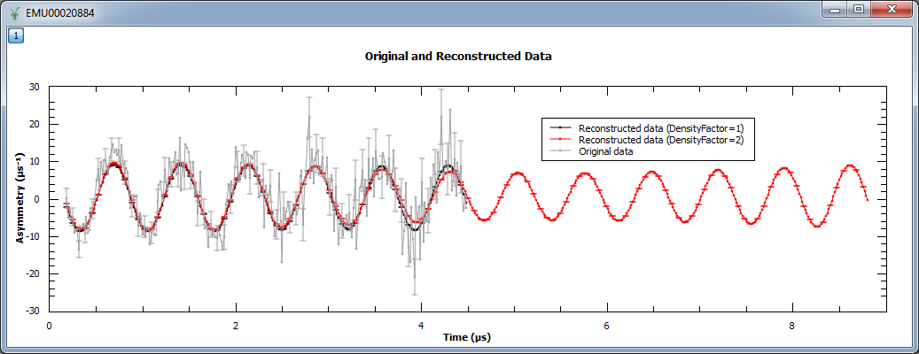
Increasing the number of points in the image ¶

The algorithm has an input property, ResolutionFactor that allows to increase the number of points in the reconstructed image. This is at present done by extending the range (and also the number of points) in the reconstructed data. The number of reconstructed points can be increased by any integer factor, but note that this will slow down the algorithm and a greater number of maxent iterations may be needed for the algorithm to converge to a solution.

An example script where the density of points is increased by a factor of 2 can be found below. Note that when a factor of 2 is used, the reconstructed data is twice the size of the original (experimental) data.

Load(Filename=r'EMU00020884.nxs', OutputWorkspace='ws')
CropWorkspace(InputWorkspace='ws', OutputWorkspace='ws', XMin=0.17, XMax=4.5, EndWorkspaceIndex=0)
ws = RemoveExpDecay(InputWorkspace='ws')
ws = Rebin(InputWorkspace='ws', Params='0.016')
evolChi1, evolAngle1, image1, data1 = MaxEnt(InputWorkspace='ws', A=0.0001, ChiTarget=300, MaxIterations=2500, ResolutionFactor=1)
evolChi2, evolAngle2, image2, data2 = MaxEnt(InputWorkspace='ws', A=0.0001, ChiTarget=300, MaxIterations=5000, ResolutionFactor=2)

print "Image at %.3f:  %.3f (ResolutionFactor=1)" % (image1.readX(0)[103], image1.readY(0)[103])
print "Image at %.3f: %.3f (ResolutionFactor=2)" % (image2.readX(0)[258], image2.readY(0)[258])

Output:

Image at -7.407:  0.000 (ResolutionFactor=1)
Image at -1.389: -0.081 (ResolutionFactor=2)

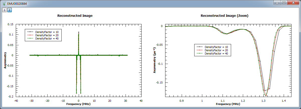
In the next example, we increased the density of points by factors of 10, 20 and 40. We show the reconstructed image (left) and a zoom into the region $0.82 < x < 1.44$ and $-0.187 < y < 0.004$ .

Load(Filename=r'EMU00020884.nxs', OutputWorkspace='ws')
CropWorkspace(InputWorkspace='ws', OutputWorkspace='ws', XMin=0.17, XMax=4.5, EndWorkspaceIndex=0)
ws = RemoveExpDecay(InputWorkspace='ws')
ws = Rebin(InputWorkspace='ws', Params='0.016')
evolChi1, evolAngle1, image1, data1 = MaxEnt(InputWorkspace='ws', A=0.0001, ChiTarget=300, MaxIterations=2500, ResolutionFactor=1)
evolChi10, evolAngle10, image10, data10 = MaxEnt(InputWorkspace='ws', A=0.0001, ChiTarget=300, MaxIterations=25000, ResolutionFactor=10)
evolChi20, evolAngle20, image20, data20 = MaxEnt(InputWorkspace='ws', A=0.0001, ChiTarget=300, MaxIterations=50000, ResolutionFactor=20)
evolChi40, evolAngle40, image40, data40 = MaxEnt(InputWorkspace='ws', A=0.0001, ChiTarget=300, MaxIterations=75000, ResolutionFactor=40)

References ¶

[1] Anders Johannes Markvardsen, (2000). Polarised neutron diffraction measurements of PrBa2Cu3O6+x and the Bayesian statistical analysis of such data. DPhil. University of Oxford (http://ora.ox.ac.uk/objects/uuid:bef0c991-4e1c-4b07-952a-a0fe7e4943f7)

[2] Skilling & Bryan, (1984). Maximum entropy image reconstruction: general algorithm. Mon. Not. R. astr. Soc. 211, 111-124.

[3] Smith & Player, (1990). Deconvolution of bipolar ultrasonic signals using a modified maximum entropy method. J. Phys. D: Appl. Phys. 24, 1714-1721.

Categories: Algorithms | Arithmetic\FFT

Source ¶

C++ source: MaxEnt.cpp

C++ header: MaxEnt.h