PDFFourierTransform dialog.
Table of Contents
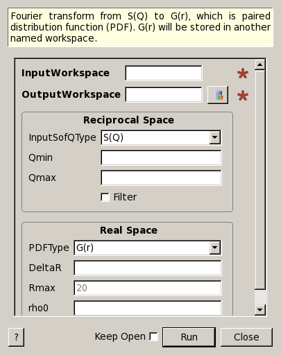
Fourier transform from S(Q) to G(r), which is paired distribution function (PDF). G(r) will be stored in another named workspace.
| Name | Direction | Type | Default | Description |
|---|---|---|---|---|
| InputWorkspace | Input | MatrixWorkspace | Mandatory | S(Q), S(Q)-1, or Q[S(Q)-1] |
| OutputWorkspace | Output | MatrixWorkspace | Mandatory | Result paired-distribution function |
| InputSofQType | Input | string | S(Q) | To identify whether input function. Allowed values: [‘S(Q)’, ‘S(Q)-1’, ‘Q[S(Q)-1]’] |
| Qmin | Input | number | Optional | Minimum Q in S(Q) to calculate in Fourier transform (optional). |
| Qmax | Input | number | Optional | Maximum Q in S(Q) to calculate in Fourier transform. (optional) |
| Filter | Input | boolean | False | Set to apply Lorch function filter to the input |
| PDFType | Input | string | G(r) | Type of output PDF including G(r). Allowed values: [‘G(r)’, ‘g(r)’, ‘RDF(r)’] |
| DeltaR | Input | number | Optional | Step size of r of G(r) to calculate. Default =  . . |
| Rmax | Input | number | 20 | Maximum r for G(r) to calculate. |
| rho0 | Input | number | Optional | Average number density used for g(r) and RDF(r) conversions (optional) |
The algorithm transforms a single spectrum workspace containing
spectral density  ,
,  , or
, or ![Q[S(Q)-1]](../_images/math/810686619f9c022ba89c00ea67318d527aeddb68.png) (as a fuction of MomentumTransfer or dSpacing units ) to a PDF
(pair distribution function) as described below.
(as a fuction of MomentumTransfer or dSpacing units ) to a PDF
(pair distribution function) as described below.
The input Workspace spectrum should be in the Q-space (MomentumTransfer) units . (d-spacing is not supported any more. Contact development team to fix that and enable dSpacing again)
Example - PDF transformation examples:
# Simulates Load of a workspace with all necessary parameters #################
import numpy as np;
xx= np.array(range(0,100))*0.1
yy = np.exp(-((xx)/.5)**2)
ws=CreateWorkspace(DataX=xx,DataY=yy,UnitX='MomentumTransfer')
Rt= PDFFourierTransform(ws,InputSofQType='S(Q)',PDFType='g(r)');
#
# Look at sample results:
print 'part of S(Q) and its correlation function'
for i in xrange(0,10):
   print '! {0:4.2f} ! {1:5f} ! {2:f} ! {3:5f} !'.format(xx[i],yy[i],Rt.readX(0)[i],Rt.readY(0)[i])
Output:
part of S(Q) and its correlation function
! 0.00 ! 1.000000 ! 0.317333 ! -3.977330 !
! 0.10 ! 0.960789 ! 0.634665 ! 2.247452 !
! 0.20 ! 0.852144 ! 0.951998 ! 0.449677 !
! 0.30 ! 0.697676 ! 1.269330 ! 1.313403 !
! 0.40 ! 0.527292 ! 1.586663 ! 0.803594 !
! 0.50 ! 0.367879 ! 1.903996 ! 1.140167 !
! 0.60 ! 0.236928 ! 2.221328 ! 0.900836 !
! 0.70 ! 0.140858 ! 2.538661 ! 1.079278 !
! 0.80 ! 0.077305 ! 2.855993 ! 0.940616 !
! 0.90 ! 0.039164 ! 3.173326 ! 1.050882 !
Categories: Algorithms | Diffraction\Utility
![G(r) = 4\pi r[\rho(r)-\rho_0] = \frac{2}{\pi} \int_{0}^{\infty} Q[S(Q)-1]\sin(Qr)dQ](../_images/math/43746d726684189b0fa241d80897c025f92aeec4.png)
![G(r) = \frac{2}{\pi} \sum_{Q_{min}}^{Q_{max}} Q[S(Q)-1]\sin(Qr) M(Q,Q_{max}) \Delta Q](../_images/math/94611d2a5221159f753f9054d3ff9d69e9cf4ed8.png)
 is an optional filter function. If Filter
property is set (true) then
is an optional filter function. If Filter
property is set (true) then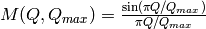
![G(r) = 4 \pi \rho_0 r [g(r)-1]](../_images/math/5a8593aaedd162c8c886ec5f565e5576b796f944.png)
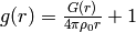

 are calculated by transforming