
PawleyFit dialog.
Table of Contents
| Name | Direction | Type | Default | Description |
|---|---|---|---|---|
| InputWorkspace | Input | MatrixWorkspace | Mandatory | Input workspace that contains the spectrum on which to perform the Pawley fit. |
| WorkspaceIndex | Input | number | 0 | Spectrum on which the fit should be performed. |
| StartX | Input | number | 0 | Lower border of fitted data range. |
| EndX | Input | number | 0 | Upper border of fitted data range. |
| LatticeSystem | Input | string | Triclinic | Lattice system to use for refinement. Allowed values: [‘Cubic’, ‘Tetragonal’, ‘Hexagonal’, ‘Rhombohedral’, ‘Orthorhombic’, ‘Monoclinic’, ‘Triclinic’] |
| InitialCell | Input | string | 1.0 1.0 1.0 90.0 90.0 90.0 | Specification of initial unit cell, given as ‘a, b, c, alpha, beta, gamma’. |
| PeakTable | Input | TableWorkspace | Mandatory | Table with peak information. Can be used instead of supplying a list of indices for better starting parameters. |
| RefineZeroShift | Input | boolean | False | If checked, a zero-shift with the same unit as the spectrum is refined. |
| PeakProfileFunction | Input | string | Gaussian | Profile function that is used for each peak. Allowed values: [‘BackToBackExponential’, ‘Bk2BkExpConvPV’, ‘DeltaFunction’, ‘ElasticDiffRotDiscreteCircle’, ‘ElasticDiffSphere’, ‘ExamplePeakFunction’, ‘Gaussian’, ‘IkedaCarpenterPV’, ‘Lorentzian’, ‘PseudoVoigt’, ‘Voigt’] |
| EnableChebyshevBackground | Input | boolean | False | If checked, a Chebyshev polynomial will be added to model the background. |
| ChebyshevBackgroundDegree | Input | number | 0 | Degree of the Chebyshev polynomial, if used as background. |
| CalculationOnly | Input | boolean | False | If enabled, no fit is performed, the function is only evaluated and output is generated. |
| OutputWorkspace | Output | MatrixWorkspace | Mandatory | Workspace that contains measured spectrum, calculated spectrum and difference curve. |
| RefinedCellTable | Output | TableWorkspace | Mandatory | TableWorkspace with refined lattice parameters, including errors. |
| RefinedPeakParameterTable | Output | TableWorkspace | Mandatory | TableWorkspace with refined peak parameters, including errors. |
| ReducedChiSquare | Output | number | Outputs the reduced chi square value as a measure for the quality of the fit. |
The algorithm performs a fit of lattice parameters using the principle approach described in a paper by Pawley [Pawley]. In this approach the reflection positions are calculated from lattice parameters and the reflection’s Miller indices ( ), while the other profile parameters for each peak are freely refined.
PawleyFit requires a MatrixWorkspace with at least one spectrum in terms of either  or
or  , the index of the spectrum can be supplied to the algorithm as a parameter. Furthermore, the range which is used for refinement can be changed by setting the corresponding properties.
In addition, a TableWorkspace with information about the reflections that are found in the spectrum must be passed as well. There must be four columns with the captions “HKL”, “d”, “FWHM (rel.)” and “Intensity”. The HKL column can be supplied either as V3D or as a string with 3 numbers separated by space, comma or semi-colon and possibly surrounded by square brackets. One way to obtain such a table is to use three algorithms that are used in analysis of POLDI data, which produce tables in a suitable format. Details are given in the usage example section.
Along with the workspaces containing fit results and parameter values, the algorithm also outputs the reduced  -value, which is also written in the log.
Note
To run these usage examples please first download the usage data, and add these to your path. In MantidPlot this is done using Manage User Directories.
For the usage example there is a calculated, theoretical diffraction pattern (including a bit of noise) for Silicon, which crystallizes in space group  and has a cubic cell with lattice parameter
 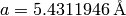 .
.
import numpy as np

# Load spectrum for Silicon in the d-range down to 0.7
si_spectrum = Load("PawleySilicon.nxs")

# In order to index the peaks later on, generate reflection for Si
Si = PoldiCreatePeaksFromCell(SpaceGroup='F d -3 m',
                              Atoms='Si 0 0 0 1.0 0.05',
                              a=5.43, LatticeSpacingMin=0.7)

print "Silicon has", Si.rowCount(), "unique reflections with d > 0.7."

# Find peaks in the spectrum
si_peaks = PoldiPeakSearch(si_spectrum)

# Index the peaks, will generate a workspace named 'si_peaks_indexed_Si'
indexed = PoldiIndexKnownCompounds(si_peaks, CompoundWorkspaces='Si')

si_peaks_indexed = AnalysisDataService.retrieve('si_peaks_indexed_Si')

# 3 peaks have two possibilities for indexing, because their d-values are identical
print "The number of peaks that were indexed:", si_peaks_indexed.rowCount()

# Run the actual fit with lattice parameters that are slightly off
si_fitted, si_cell, si_params, chi_square = PawleyFit(si_spectrum,
                      LatticeSystem='Cubic',
                      InitialCell='5.436 5.436 5.436',
                      PeakTable=si_peaks_indexed)

si_cell = AnalysisDataService.retrieve("si_cell")

a = np.round(si_cell.cell(0, 1), 6)
a_err = np.round(si_cell.cell(0, 2), 6)
a_diff = np.round(np.fabs(a - 5.4311946), 6)

print "The lattice parameter was refined to a =", a, "+/-", a_err
print "The deviation from the actual parameter (a=5.4311946) is:", a_diff
print "This difference corresponds to", np.round(a_diff / a_err, 2), "standard deviations."
print "The reduced chi square of the fit is:", np.round(chi_square, 3)
Running this script will generate a bit of output about the results of the different steps. At the end the lattice parameter differs less than one standard deviation from the actual value.
Silicon has 18 unique reflections with d > 0.7.
The number of peaks that were indexed: 15
The lattice parameter was refined to a = 5.431205 +/- 1.6e-05
The deviation from the actual parameter (a=5.4311946) is: 1e-05
This difference corresponds to 0.63 standard deviations.
The reduced chi square of the fit is: 1.04
It’s important to check the output data, which is found in the workspace labeled si_fitted. Plotting it should show that the residuals are just containing background noise and no systematic deviations. Of course, depending on the sample and the measurement this will differ between cases.
Result of the Pawley fit example with silicon.
| [Pawley] | Pawley, G. S. “Unit-Cell Refinement from Powder Diffraction Scans.”, J. Appl. Crystallogr. 14, 1981, 357. doi:10.1107/S0021889881009618. |
Categories: Algorithms | Diffraction\Fitting