Calibration is currently based on tubes and is accessed using the tube module.
excludeShorTubes, overridePeaks, fitPolyn, outputPeak ] )
Among the examples, inside the Examples folder, the user is encouraged to look at TubeCalibDemoMaps_All, there he will find 7 examples showing how to use calibrate method.
Tube Calibration Demonstration for MAPS instrument.
This module group many examples and also demonstrate how to work with the tube.calibrate().
It starts from the simplest way to perform a calibration. It them increase the complexity of dealing with real calibration work, when particularities of the instrument must be considered
At the end, it gives a suggestion on a techinique to investigate and improve the calibration itself.
Simplest way of calling tube.calibrate()
The minimal input for the calibration is the integrated workspace and the knwon positions.
Eventhough it is easy to call, the calibration performs well, but there are ways to improve the results, as it is explored after.
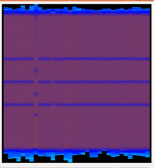
Giving the expected value for the position of the peaks in pixel.
The minimalInput() let to the calibrate to guess the position of the pixels among the tubes. Altough it works nicelly, providing these expected values may improve the results. This is done through the fitPar parameter.
To fit correcly, it is important to have a good window around the peak. This windown is defined by the margin parameter.
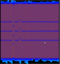
This examples shows how the results worsen if we change the margin from its default value 15 to 10.
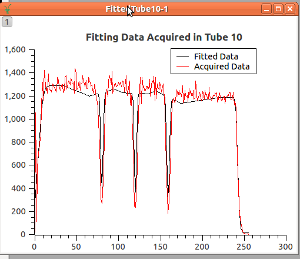
It shows how to see the fitted values using the plotTube parameter.
It will also output the peaks position and save them, through the outputPeak option and the tube.savePeak() method.
An example of the fitted data compared to the acquired data to find the peaks positions:
The result deteriorate, as you can see:
The provideTheExpectedValue() provided a good solution, but there are few tubes whose calibration was not so good.
This method explores how to deal with these tubes.
First of all, it is important to identify the tubes that did not work well.
From the outputs of provideTheExpectedValue, looking inside the instrument tree, it is possible to list all the tubes that are not so good.
Unfortunatelly, they do not have a single name identifier. So, locating them it is a little bit trickier. The findThoseTubesThatNeedSpecialCareForCalibration() shows one way of finding those tubes. The index is the position inside the PeakTable.
For this example, we have used inspection from the Instrument View. One of them is inside the A1_Window, 3rd PSD_TUBE_STRIP 8 pack up, 4th PSD_TUBE_STRIP: Index = 8+8+4 - 1 = 19.
In this example, we will ask the calibration to run the calibration only for 3 tubes (indexes 18,19,20). Them, we will check why the 19 is not working well. Finally, we will try to provide another peaks position for this tube, and run the calibration again for these tubes, to improve the results.
This example shows how to use overridePeaks option
Analysing the result of provideTheExpectedValue it was seen that the calibration of some tubes was not good.
Note
This method list some of them, there are a group belonging to window B2 that shows only 2 peaks that are not dealt with here.
If first plot the bad ones using the plotTube option. It them, find where they fail, and how to correct their peaks, using the overridePeaks. If finally, applies the calibration again with the points corrected.
There are among the B2 window tubes, some tubes that are showing only 2 strips.
Those tubes must be calibrated separated, as the known positions are not valid.
This example calibrate them, using only 4 known values: 2 edges and 2 peaks.
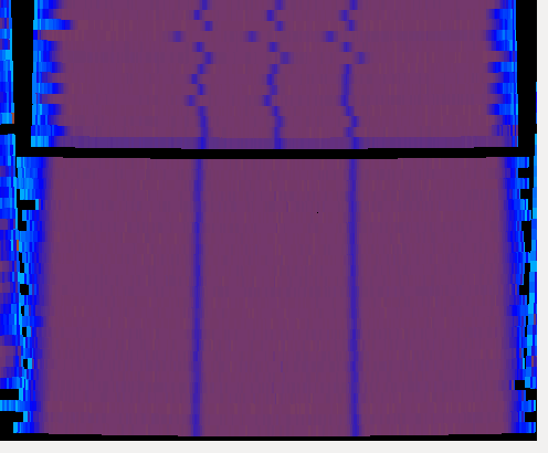
Run this example, and them see the worksapce in the calibrated instrument and you will see how it worked.
The picture shows the output, look that only a section of the B2 Window was calibrated.
This example shows how to use some properties of calibrate method to join together the calibration done in provideTheExpectedValue(), and improved in calibrateB2Window(), and improvingCalibrationOfListOfTubes().
It also improves the result of the calibration because it deals with the E door. The aquired data cannot be used to calibrate the E door, and trying to do so, produces a bad result. In this example, the tubes inside the E door are excluded to the calibration. Using the ‘’‘rangeList’‘’ option.
The example provideTheExpectedValue() has shown its capability to calibrate almost all tubes, but, as explored in the improvingCalibrationOfListOfTubes() and improvingCalibrationSingleTube() there are some tubes that could not be calibrated using that method.
The goal of this method is to show one way to find the tubes that will require special care.
It will first perform the same calibration seen in provideTheExpectedValue(), them, it will process the peakTable output of the calibrate method when enabling the parameter outputPeak.
It them creates the Peaks workspace, that is the diffence of the peaks position from the expected values of the peaks positions for all the tubes. This allows to spot what are the tubes whose fitting are outliers in relation to the others.
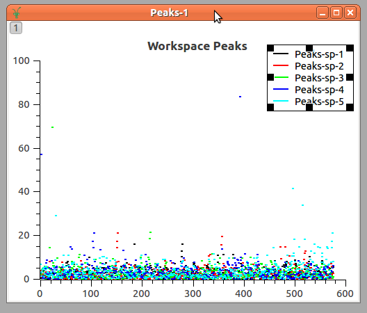
The final result for this method is to output using plotTube the result of the fitting to all the ‘outliers’ tubes.
Tube Calibration Demonstration program for MERLIN.
Attention
MERLIN instruments are loaded with already calibrated values. The calibration works nicelly with these files, but if you want to see the uncalibrated file you can do it. Look at How to reset detectors calibration.
In this example, the calibration of the whole MERLIN instrument is shown. It demonstrate how to use tube.calibrate() to calibrate MERLIN tubes.
Opening the calibrated data in the Instrument View, it is possible to group the tubes in some common regions:
This example shows:
- How to calibrate regions of the instrument separetelly.
- How to use calibTable parameter to append information in order to create a calibration table for the whole instrument.
- How to use the outputPeak to check how the calibration is working as well as the usage of analisePeakTable method to look into the details of the operation to improve the calibration.
- It deals with defining different known positions for the different tube lengths.
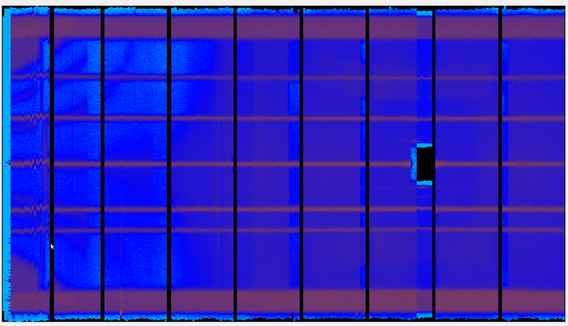
The output of this examples shows an improvement in relation to the previous calibrated instrument.
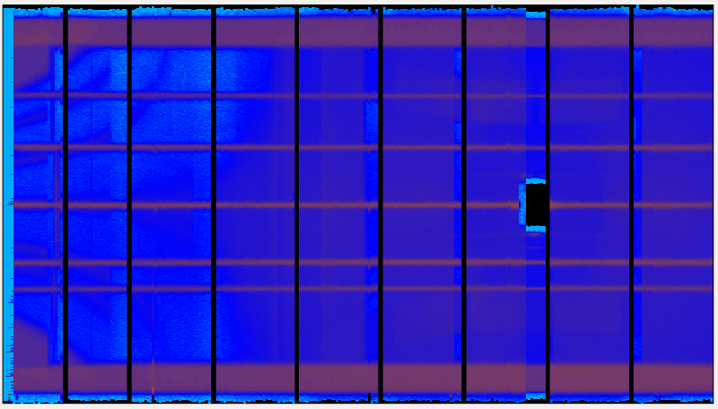
The previous calibrated instrument view:
Allows to save the peakTable to a text file.
| Parameters: | peakTable – peak table as the workspace table provided by calibrated method, as in the example: |
|---|
calibTable, peakTable = calibrate(..., outputPeak=peakTable)
savePeak(peakTable, 'myfolder/myfile.txt')
| Parameters: | filePath – where to save the file. If the filePath is not given as an absolute path, it will be considered relative to the defaultsave.directory. |
|---|
The file will be saved with the following format:
id_name (parsed space to %20) [peak1, peak2, ..., peakN]
You may load these peaks using readPeakFile
panel1/tube001 [23.4, 212.5, 0.1]
...
panel1/tubeN   [56.3, 87.5, 0.1]
Load the file calibration
It returns a list of tuples, where the first value is the detector identification and the second value is its calibration values.
Example of usage:
for (det_code, cal_values) in readPeakFile('pathname/TubeDemo'):
   print det_code
   print cal_values
| Parameters: | file_name – Path for the file |
|---|---|
| Return type: | list of tuples(det_code, peaks_values) |
More details on the finer points of the calibration implementation can be found at http://www.mantidproject.org/Tube_Calibration and in: