There is direct support for defining any of the following geometric shapes to add Instrument Definition File.
In addition to the shapes listed above, other shapes may be defined by combining already defined shapes into new ones. This is done using an algebra that follows the following notation:
| Operator | Description | Example |
|---|---|---|
| : | Union (i.e two or more things making up one shape). See e.g. also 1 | a body = legs : torso : arms : head |
| ” “ | “space” shared between shapes, i,e. intersection (the common region of shapes). See e.g. also 2 | “small-circle = big-circle small-circle” (where the small circle placed within the big-circle) |
| # | Complement | # sphere = shape defined by all points outside sphere |
| ( ) | Brackets are used to emphasise which shapes an operation should be applied to. | box1 (# box2) is the intersection between box1 and the shape defined by all points not inside box2 |
All objects are defined with respect to cartesian axes (x,y,z), and the default unit of all supplied values are metres(m). Objects may be defined so that the origin (0,0,0) is at the centre, so that when rotations are applied they do not also apply an unexpected translation.
Within instrument definitions we support the concept of defining a rotation by specifying what point the object is facing. To apply that correctly the side of the object we consider to be the front is the xy plane. Hence, when planning to use facing the shape should be defined such that the positive y-axis is considered to be up, the x-axis the width, and the z-axis the depth of the shape.
When defining a shape you have complete freedom to define it with respect to whatever coordinate system you like. However, we have a least the following recommendation
<sphere id="some-sphere">
  <centre x="0.0"  y="0.0" z="0.0" />
  <radius val="0.5" />
</sphere>

<algebra val="some-sphere" />
Any shape must be given an ID name. Here the sphere has been given the name “some-sphere”. The purpose of the ID name is to use it in the description, here this is done with the line . The description is optional. If it is left out the algebraic intersection is taken between any shapes defined.
<cylinder id="stick">
  <centre-of-bottom-base x="-0.5" y="0.0" z="0.0" />
  <axis x="1.0" y="0.0" z="0.0" />
  <radius val="0.05" />
  <height val="1.0" />
</cylinder>

<sphere id="some-sphere">
  <centre x="0.0"  y="0.0" z="0.0" />
  <radius val="0.5" />
</sphere>

<algebra val="some-sphere (# stick)" />
This algebra string reads as follows: take the intersection between a sphere and the shape defined by all points not inside a cylinder of length 1.0 along the x-axis. Note the brackets around # stick in the algebraic string are optional, but here included to emphasis that the “space” between the “some-sphere” and “(# stick)” is the intersection operator.
<sphere id="A">
  <centre x="4.1"  y="2.1" z="8.1" />
  <radius val="3.2" />
</sphere>
<cylinder id="A">
  <centre-of-bottom-base r="0.0" t="0.0" p="0.0" />  <!-- here position specified using spherical coordinates -->
  <axis x="0.0" y="0.2" z="0" />
  <radius val="1" />
  <height val="10.2" />
</cylinder>
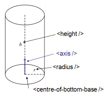
Schematic of a cylinder
<hollow-cylinder id="A">
  <centre-of-bottom-base r="0.0" t="0.0" p="0.0" />  <!-- here position specified using spherical coordinates -->
  <axis x="0.0" y="1.0" z="0" />
  <inner-radius val="0.007" />
  <outer-radius val="0.01" />
  <height val="0.05" />
</hollow-cylinder>
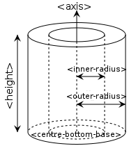
Schematic of a hollow cylinder
<infinite-cylinder id="A" >
  <centre x="0.0" y="0.2" z="0" />
  <axis x="0.0" y="0.2" z="0" />
  <radius val="1" />
</infinite-cylinder>
<slice-of-cylinder-ring id="A">
  <inner-radius val="0.0596"/>
  <outer-radius val="0.0646"/>
  <depth val="0.01"/>
  <arc val="45.0"/>
</slice-of-cylinder-ring>
This XML element defines a slice of a cylinder ring. Most importantly the part of this shape facing the sample is flat and looks like this:
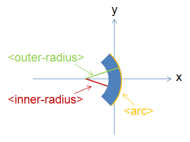
XMLsliceCylinderRingDescription.png
<cone id="A" >
  <tip-point x="0.0" y="0.2" z="0" />
  <axis x="0.0" y="0.2" z="0" />
  <angle val="30.1" />
  <height val="10.2" />
</cone>
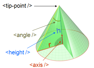
XMLconeDescription.png
<infinite-cone id="A" >
  <tip-point x="0.0" y="0.2" z="0" />
  <axis x="0.0" y="0.2" z="0" />
  <angle val="30.1"  />
</infinite-cone>
Is the 3D shape of all points on the plane and all points on one side of the infinite plane, the side which point away from the infinite plane in the direction of the normal vector.
<infinite-plane id="A">
  <point-in-plane x="0.0" y="0.2" z="0" />
  <normal-to-plane x="0.0" y="0.2" z="0" />
</infinite-plane>
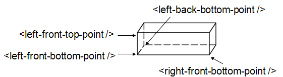
<cuboid id="shape">
  <left-front-bottom-point x="0.0025" y="-0.1" z="0.0"  />
  <left-front-top-point  x="0.0025" y="-0.1" z="0.02"  />
  <left-back-bottom-point  x="-0.0025" y="-0.1" z="0.0"  />
  <right-front-bottom-point  x="0.0025" y="0.1" z="0.0"  />
</cuboid>
<algebra val="shape" />
This particular example describes a cuboid with the origin at the centre of the front face, which is here facing the negative z-axis and has the dimensions 0.005mm x 0.2mm (in the xy-plane), and the depth of this cuboid is 0.02mm.
XMLcuboidDescription.png
Another example of a cuboid is
<cuboid id="shape">
  <left-front-bottom-point x="0.0" y="-0.1" z="-0.01"  />
  <left-front-top-point  x="0.0" y="0.1" z="-0.01"  />
  <left-back-bottom-point  x="0.001" y="-0.1" z="-0.01"  />
  <right-front-bottom-point  x="0.0" y="-0.1" z="0.01"  />
</cuboid>
<algebra val="shape" />
which describes a cuboid with a front y-z plane (looking down the x-axis). The origin is assumed to be the centre of this front surface, which has dimensions 200mm along y and 20mm along z. The depth of this cuboid is taken to be 1mm (along x).
<hexahedron id="Bertie">
  <left-back-bottom-point  x="0.0" y="0.0" z="0.0"  />
  <left-front-bottom-point x="1.0" y="0.0" z="0.0"  />
  <right-front-bottom-point x="1.0" y="1.0" z="0.0"  />
  <right-back-bottom-point  x="0.0" y="1.0" z="0.0"  />
  <left-back-top-point  x="0.0" y="0.0" z="2.0"  />
  <left-front-top-point  x="0.5" y="0.0" z="2.0"  />
  <right-front-top-point  x="0.5" y="0.5" z="2.0"  />
  <right-back-top-point  x="0.0" y="0.5" z="2.0"  />
</hexahedron>
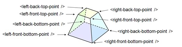
XMLhexahedronDescription.png
Available from version 3.0 onwards.
A tapered guide is a special case of hexahedron; a “start” rectangular aperture which in a continued fashion changes into an “end” rectangular aperture.
<tapered-guide id="A Guide">
    <aperture-start height="2.0" width="2.0" />
    <length val="3.0" />
    <aperture-end height="4.0" width="4.0" />
    <centre x="0.0" y="5.0" z="10.0" /> <!-- Optional.  Defaults to (0, 0 ,0) -->
    <axis x="0.5" y="1.0" z="0.0" /> <!-- Optional.  Defaults to (0, 0 ,1) -->
</tapered-guide>
The centre value denotes the centre of the start aperture. The specified axis runs from the start aperture to the end aperture. “Height” is along the y-axis and “width” runs along the x-axis, before the application of the “axis” rotation.
When a geometric shape is rendered in the MantidPlot instrument viewer, Mantid will attempt to automatically construct an axis-aligned bounding box for every geometric shape that does not have one yet. Well-defined bounding boxes are required by many features of Mantid, from correctly rendering the instrument to performing calculations in various algorithms.
The automatically calculated bounding boxes can generally be relied upon and are usually ideal. However, if the automatic calculation fails to produce a reasonable bounding box, or if performance becomes an issue with particularly complex shapes, you have the option of adding a manually pre-calculated bounding box.
A typical symptom of the automatic calculation creating an incorrect bounding box is your instrument appearing very small when viewed (forcing you to zoom in for a long time to see it). In such cases, the axis visualizations also tend to not display properly.
A custom bounding-box can be added to shapes using the following notation:
<hexahedron id="shape">
  <left-front-bottom-point x="0.0" y="-0.037" z="-0.0031"  />
  <right-front-bottom-point x="0.0" y="-0.037" z="0.0031"  />
  <left-front-top-point x="0.0" y="0.037" z="-0.0104"  />
  <right-front-top-point x="0.0" y="0.037" z="0.0104"  />
  <left-back-bottom-point x="0.005" y="-0.037" z="-0.0031"  />
  <right-back-bottom-point x="0.005" y="-0.037" z="0.0031"  />
  <left-back-top-point x="0.005" y="0.037" z="-0.0104"  />
  <right-back-top-point x="0.005" y="0.037" z="0.0104"  />
</hexahedron>
<algebra val="shape" />

<bounding-box>
  <x-min val="0.0"/>
  <x-max val="0.005"/>
  <y-min val="-0.037"/>
  <y-max val="0.037"/>
  <z-min val="-0.0104"/>
  <z-max val="0.0104"/>
</bounding-box>
Note for the best effect this bounding box should be enclosing the shape as tight as possible.
Category: Concepts