Indirect Corrections¶

Table of Contents

Overview
- Action Buttons
Calculate Paalman Pings
- Options
- Shape Details
- Background
Apply Paalman Pings
- Options
Absorption Corrections
Container Subtraction
- Options

Overview ¶

Provides correction routines for quasielastic, inelastic and diffraction reductions.

Action Buttons ¶

?: Opens this help page.
Py: Exports a Python script which will replicate the processing done by the current tab.
Run: Runs the processing configured on the current tab.
Manage Directories: Opens the Manage Directories dialog allowing you to change your search directories and default save directory and enable/disable data archive search.

Calculate Paalman Pings ¶

Calculates absorption corrections in the Paalman & Pings absorption factors that could be applied to the data when given information about the sample (and optionally can) geometry.

Options ¶

Input: Either a reduced file (_red.nxs) or workspace (_red) or an $S(Q, \omega)$ file (_sqw.nxs) or workspace (_sqw).
Use Can: If checked allows you to select a workspace for the container in the format of either a reduced file (_red.nxs) or workspace (_red) or an $S(Q, \omega)$ file (_sqw.nxs) or workspace (_sqw).
Sample Shape: Sets the shape of the sample, this affects the options for the shape details (see below).
Sample/Can Number Density: Density of the sample or container.
Sample/Can Chemical Formula: Chemical formula of the sample or can material. This must be provided in the format expected by the SetSampleMaterial algorithm.
Plot Output: Plots the $A_{s,s}$ , $A_{s,sc}$ , $A_{c,sc}$ and $A_{c,c}$ workspaces as spectra plots.
Save Result: If enabled the result will be saved as a NeXus file in the default save directory.

Shape Details ¶

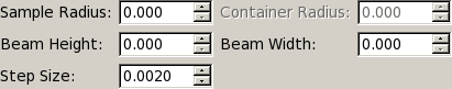
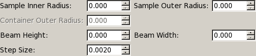
Depending on the shape of the sample different parameters for the sample dimension are required and are detailed below.

Flat Plate ¶

The calculation for a flat plate geometry is performed by the FlatPlatePaalmanPingsCorrection algorithm.

Sample Thickness: Thickness of sample in $cm$ .
Sample Angle: Sample angle in degrees.
Can Front Thickness: Thickness of front container in $cm$ .
Can Back Thickness: Thickness of back container in $cm$ .

The calculation for a cylindrical geometry is performed by the CylinderPaalmanPingsCorrection algorithm, this algorithm is currently only available on Windows as it uses FORTRAN code dependant of F2Py.

Sample Inner Radius: Radius of the inner wall of the sample in $cm$ .
Sample Outer Radius: Radius of the outer wall of the sample in $cm$ .
Container Outer Radius: Radius of outer wall of the container in $cm$ .
Beam Height: Height of incident beam $cm$ .
Beam Width: Width of incident beam in $cm$ .
Step Size: Step size used in calculation.

Annulus ¶

The calculation for an annular geometry is performed by the CylinderPaalmanPingsCorrection algorithm, this algorithm is currently only available on Windows as it uses FORTRAN code dependant of F2Py.

The options here are the same as for Cylinder.

Background ¶

The main correction to be applied to neutron scattering data is that for absorption both in the sample and its container, when present. For flat plate geometry, the corrections can be analytical and have been discussed for example by Carlile [1]. The situation for cylindrical geometry is more complex and requires numerical integration. These techniques are well known and used in liquid and amorphous diffraction, and are described in the ATLAS manual [2].

The absorption corrections use the formulism of Paalman and Pings [3] and involve the attenuation factors $A_{i,j}$ where $i$ refers to scattering and $j$ attenuation. For example, $A_{s,sc}$ is the attenuation factor for scattering in the sample and attenuation in the sample plus container. 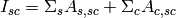If the scattering cross sections for sample and container are $\Sigma_{s}$ and $\Sigma_{c}$ respectively, then the measured scattering from the empty container is $I_{c} = \Sigma_{c}A_{c,c}$ and that from the sample plus container is $I_{sc} = \Sigma_{s}A_{s,sc} + \Sigma_{c}A_{c,sc}$ , thus $\Sigma_{s} = (I_{sc} - I_{c}A_{c,sc}/A_{c,c}) / A_{s,sc}$ .

References:

C J Carlile, Rutherford Laboratory report, RL-74-103 (1974)
A K Soper, W S Howells & A C Hannon, RAL Report RAL-89-046 (1989)
H H Paalman & C J Pings, J Appl Phys 33 2635 (1962)

Apply Paalman Pings ¶

The Apply Corrections tab applies the corrections calculated in the Calculate Corrections tab of the Indirect Data Analysis interface.

This uses the ApplyPaalmanPingsCorrection algorithm to apply absorption corrections in the form of the Paalman & Pings correction factors. When Use Can is disabled only the $A_{s,s}$ factor must be provided, when using a container the additional factors must be provided: $A_{c,sc}$ , $A_{s,sc}$ and $A_{c,c}$ .

Once run the corrected output and can correction is shown in the preview plot, the Spectrum spin box can be used to scroll through each spectrum. Note that when this plot shows the result of a calculation the X axis is always in wavelength, however when data is initially selected the X axis unit matches that of the sample workspace.

The input and container workspaces will be converted to wavelength (using ConvertUnits) if they do not already have wavelength as their X unit.

The binning of the sample, container and corrections factor workspace must all match, if the sample and container do not match you will be given the option to rebin (using RebinToWorkspace) the sample to match the container, if the correction factors do not match you will be given the option to interpolate (SplineInterpolation) the correction factor to match the sample.

Options ¶

Input: Either a reduced file (_red.nxs) or workspace (_red) or an $S(Q, \omega)$ file (_sqw.nxs) or workspace (_sqw).
Geometry: Sets the sample geometry (this must match the sample shape used when running Calculate Corrections).
Use Can: If checked allows you to select a workspace for the container in the format of either a reduced file (_red.nxs) or workspace (_red) or an $S(Q, \omega)$ file (_sqw.nxs) or workspace (_sqw).
Scale Can by factor: Allows the container intensity to be scaled by a given scale factor before being used in the corrections calculation.
Use Corrections: The Paalman & Pings correction factors to use in the calculation, note that the file or workspace name must end in either _flt_abs or _cyl_abs for the flat plate and cylinder geometries respectively.
Plot Output: Gives the option to create either a spectra or contour plot (or both) of the corrected workspace.
Save Result: If enabled the result will be saved as a NeXus file in the default save directory.

Absorption Corrections ¶

The Absorption Corrections tab provides a cross platform alternative to the previous Calculate and Apply Corrections tabs.

Common Options ¶

Sample Input: Used to select the sample from either a file or a workspace already loaded into Mantid.
Use Container: Used to enable or disable use of a container and selects one from either a file or loaded workspace.
Shape: Select the shape of the sample (see specific geometry options below).
Number Density: Number density for either the sample or container.
Chemical Formula: Chemical formula for either the sample or container in the format expected by SetSampleMaterial.
Use Container Corrections: Enables full container corrections, if disabled only a can subtraction will be performed.
Scale: Scale factor to scale container input by.
Keep Correction Factors: If checked a Workspace Group containing the correction factors will also be created, this will have the suffix _Factors.
Plot Result: If checked the corrected workspace and correction factors will be plotted.
Save Result: If checked the corrected workspace and (if Keep Correction Factors is checked) the correction factor workspace will be saved as a NeXus file in the default save directory.

Flat Plate ¶

Flat plate calculations are provided by the IndirectFlatPlateAbsorption algorithm.

Sample Width: Width of the sample in $cm$ .
Sample Height: Height of the sample in $cm$ .
Sample Thickness: Thickness of the sample in $cm$ .
Container Front Thickness: Thickness of the front of the container in $cm$ .
Container Back Thickness: Thickness of the back of the container in $cm$ .
Element Size: Size of the square “chunks” to divide the frontal area of the sample into to calculate corrections in $cm$ .

Annulus ¶

Annulus calculations are provided by the IndirectAnnulusAbsorption algorithm.

Sample Inner Radius: Radius of the inner wall of the sample in $cm$ .
Sample Outer Radius: Radius of the outer wall of the sample in $cm$ .
Container Inner Radius: Radius of the inner wall of the container in $cm$ .
Container Outer Radius: Radius of the outer wall of the container in $cm$ .
Neutron Events: Number of events to use in the Monte Carlo simulation.

Cylinder ¶

Cylinder calculations are provided by the IndirectCylinderAbsorption algorithm.

Sample Radius: Radius of the outer wall of the sample in $cm$ .
Container Radius: Radius of the outer wall of the container in $cm$ .
Neutron Events: Number of events to use in the Monte Carlo simulation.

Container Subtraction ¶

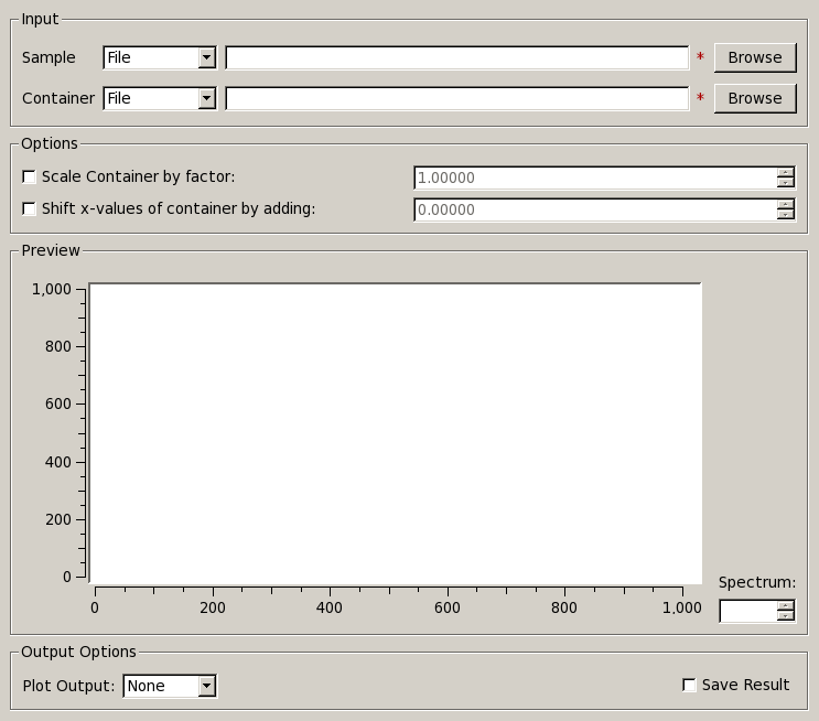
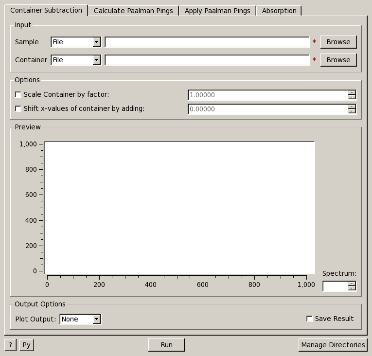
The Container Subtraction Tab is used to remove the containers contribution to a run.

The input and container workspaces will be converted to wavelength (using ConvertUnits) if they do not already have wavelength as their X unit.

Options ¶

Input Sample: Either a reduced file (_red.nxs) or workspace (_red) or an S(Q,omega) file (_sqw.nxs) or workspace (_sqw) that represents the sample.
Input Container: Either a reduced file (_red.nxs) or workspace (_red) or an S(Q,omega) file (_sqw.nxs) or workspace (_sqw) that represents the container.
Scale Can by Factor: Allows the container intensity to be scaled by a given scale factor before being used in the corrections calculation.
Plot Output: Gives the option to create either a spectra or contour plot (or both) of the corrected workspace.
Save Result: If enabled the result will be saved as a NeXus file in the default save directory.

Categories: Interfaces | Indirect