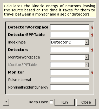
GetEiMonDet dialog.
Table of Contents
Calculates the kinetic energy of neutrons leaving the source based on the time it takes for them to travel between a monitor and a set of detectors.
| Name | Direction | Type | Default | Description |
|---|---|---|---|---|
| DetectorWorkspace | Input | MatrixWorkspace | Mandatory | A workspace containing the detector spectra. |
| DetectorEPPTable | Input | TableWorkspace | Mandatory | An EPP table corresponding to DetectorWorkspace. |
| IndexType | Input | string | DetectorID | The type of indices Detectors and Monitor refer to. Allowed values: [‘DetectorID’, ‘SpectrumNumber’, ‘WorkspaceIndex’] |
| Detectors | Input | string | Mandatory | A list of detector ids/spectrum number/workspace indices. |
| MonitorWorkspace | Input | MatrixWorkspace | A Workspace containing the monitor spectrum. If empty, DetectorWorkspace will be used. | |
| MonitorEPPTable | Input | TableWorkspace | An EPP table corresponding to MonitorWorkspace | |
| Monitor | Input | number | Mandatory | Monitor’s detector id/spectrum number/workspace index. |
| PulseInterval | Input | number | Optional | Interval between neutron pulses, in microseconds. |
| NominalIncidentEnergy | Input | number | Optional | Incident energy guess. Taken from the sample logs, if not specified. |
| IncidentEnergy | Output | number | Calculated incident energy. |
This algorithm calculates the incident energy from the time-of-flight between one monitor and some detectors. The time information is extracted from the PeakCentre columns of the EPP workspaces. The FitSuccess column in the EPP tables is used to single out detectors without good quality elastic peaks: only detectors with success in the column are accepted. Monitor-to-sample and sample-to-detector distances are loaded from the instrument definition. Both the time and the distance data is averaged over the specified detectors.
The EPP tables can be produced using the FindEPP v1 algorithm.
If no MonitorWorkspace is specified, the monitor spectrum is expected to be in the detector workspace.
The drop-down menu is used to specify what the numbers in the Detectors and Monitor fields mean. The Detectors field understands complex expression, for example 2,3,5-7,101 would use detectors 2, 3, 5, 6, 7, and 101 for the computation.
It is possible that a neutron pulse is detected at the detectors in a later frame than at the monitor. These cases can be identified if the time-of-flight from the monitor to the detectors is negative or if the calculated incident energy would end up being too large. In these cases, the value of the PulseInterval field is added to the time-of-flight until the result is satisfactory.
To identify when the incident energy is within acceptable bounds, the algorithm applies simple heuristics. Basically, the final energy has to be within 20% of the NominalIncidentEnergy or within the PulseInterval corrected time-of-flight  PulseInterval / 2.
Example - simple incident energy calibration:
import numpy
from scipy.constants import elementary_charge, neutron_mass

# We need some definitions for a fake instrument and data.
# Nominal (ideal) incident energy, in meV.
E_i = 55.0
# In reality, the energy is something else.
realE_i = 0.98 * E_i
# Position of peaks in microseconds.
# Has to be the same for monitor and detectors because of
# the way the fake instrument is created. This also implies
# that the neutron pulse will arrive at the detectors in the
# next frame.
peakPosition = 300.0
pulseInterval = 1500.0
# Specify/calculate instrument dimensions.
monitorToSample = 0.6
# Remember, the neutrons are detected in the next frame.
timeOfFlight = pulseInterval
velocity = numpy.sqrt(2 * realE_i * elementary_charge * 1e-3 / neutron_mass)
sampleToDetector = velocity * timeOfFlight * 1e-6 - monitorToSample

# Fake workspace creation. This is a bit ugly hack, but we
# will create a workspace with two detector banks and eventually
# move one of them where the monitor is supposed to be pretending
# that it actually is the monitor.

# First the spectra. They contain a single peak at peakPosition.
spectrum = 'name = Gaussian, PeakCentre = {0}, Height = 500.0, Sigma = 30.0'.format(peakPosition)
# The workspace itself.
ws = CreateSampleWorkspace(WorkspaceType = 'Histogram', XUnit = 'TOF',\
XMin = 100.0, XMax = 1100.0, BinWidth = 10.0,\
NumBanks = 2, BankDistanceFromSample = sampleToDetector,\
Function = 'User Defined', UserDefinedFunction = spectrum)
# Move the detector.
MoveInstrumentComponent(Workspace = ws, ComponentName = 'basic_rect/bank2',\
X = -monitorToSample,\
RelativePosition = False)

# Preparations are done, actual calibration ensues.
eppTable = FindEPP(InputWorkspace = ws)
# We choose all detectors in the detector bank, and only the
# centre detector as the monitor in the monitor bank.
calibratedE_i = GetEiMonDet(DetectorWorkspace = ws, DetectorEPPTable = eppTable,\
Detectors = "100-199", Monitor = 200,\
NominalIncidentEnergy = E_i, PulseInterval = pulseInterval)

print('Nominal incident energy: {0:.5f}'.format(E_i))
print('Calibrated energy: {0:.5f}'.format(calibratedE_i))
print('Real energy: {0:.5f}'.format(realE_i))
Output:
Nominal incident energy: 55.00000
Calibrated energy: 53.90968
Real energy: 53.90000
Categories: Algorithms | Inelastic\Ei