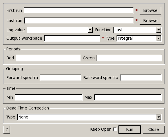
PlotAsymmetryByLogValue dialog.
Table of Contents
| Name | Direction | Type | Default | Description |
|---|---|---|---|---|
| FirstRun | Input | string | Mandatory | The name of the first workspace in the series. Allowed extensions: [‘.nxs’] |
| LastRun | Input | string | Mandatory | The name of the last workspace in the series. Allowed extensions: [‘.nxs’] |
| OutputWorkspace | Output | MatrixWorkspace | Mandatory | The name of the output workspace containing the resulting asymmetries. |
| LogValue | Input | string | Mandatory | The name of the log values which will be used as the x-axis in the output workspace. |
| Function | Input | string | Last | The function to apply: ‘Mean’, ‘Min’, ‘Max’, ‘First’ or ‘Last’. Allowed values: [‘Mean’, ‘Min’, ‘Max’, ‘First’, ‘Last’] |
| Red | Input | number | 1 | The period number for the ‘red’ data. |
| Green | Input | number | Optional | The period number for the ‘green’ data. |
| Type | Input | string | Integral | The calculation type: ‘Integral’ or ‘Differential’. Allowed values: [‘Integral’, ‘Differential’] |
| TimeMin | Input | number | Optional | The beginning of the time interval used in the calculations. |
| TimeMax | Input | number | Optional | The end of the time interval used in the calculations. |
| ForwardSpectra | Input | int list | The list of spectra for the forward group. If not specified the following happens. The data will be grouped according to grouping information in the data, if available. The forward will use the first of these groups. | |
| BackwardSpectra | Input | int list | The list of spectra for the backward group. If not specified the following happens. The data will be grouped according to grouping information in the data, if available. The backward will use the second of these groups. | |
| DeadTimeCorrType | Input | string | None | Type of Dead Time Correction to apply. Allowed values: [‘None’, ‘FromRunData’, ‘FromSpecifiedFile’] |
| DeadTimeCorrFile | Input | string | Custom file with Dead Times. Will be used only if appropriate DeadTimeCorrType is set. Allowed extensions: [‘.nxs’] |
This algorithm calculates asymmetry for a series of Muon workspaces. The input workspaces must be in Muon Nexus files, the names of which follow the rule: the filename must begin with at least 1 letter and followed by a number. The input property FirstRun must be set to the file name with the smallest number and the LastRun to the one with the highest number.
The output workspace contains asymmetry as the Y values, and the selected log values for X. The log values can be chosen as the mean, minimum, maximum, first or last if they are a time series. For start/end times, the values are in seconds relative to the start time of the first run.
If the “Green” property is not set the output workspace will contain a single spectrum with asymmetry values. If the “Green” is set the output workspace will contain four spectra with asymmetries:
| Workspace Index | Spectrum | Asymmetry |
|---|---|---|
| 0 | 1 | Difference of Red and Green |
| 1 | 2 | Red only |
| 2 | 3 | Green only |
| 3 | 4 | Sum of Red and Green |
If ForwardSpectra and BackwardSpectra are set the Muon workspaces will be grouped according to the user input, otherwise the Autogroup option of LoadMuonNexus will be used for grouping.
Note
To run these usage examples please first download the usage data, and add these to your path. In MantidPlot this is done using Manage User Directories.
Example - Calculating asymmetry for a series of MUSR runs:
ws = PlotAsymmetryByLogValue(FirstRun = 'MUSR00015189.nxs',
                             LastRun = 'MUSR00015191.nxs',
                             LogValue = 'sample_magn_field',
                             TimeMin = 0.55,
                             TimeMax = 12.0);

print "Y values (asymmetry):", ws.readY(0)
print "X values (sample magn. field):", ws.readX(0)
Output:
Y values (asymmetry): [ 0.14500665  0.136374    0.11987909]
X values (sample magn. field): [ 1350.  1360.  1370.]
Example - Using both Red and Green periods:
ws = PlotAsymmetryByLogValue(FirstRun = 'MUSR00015189.nxs',
                             LastRun = 'MUSR00015191.nxs',
                             LogValue = 'sample_magn_field',
                             TimeMin = 0.55,
                             TimeMax = 12.0,
                             Red = 1,
                             Green = 2);

print "Y values (difference):", ws.readY(0)
print "Y values (red):", ws.readY(1)
print "Y values (green):", ws.readY(2)
print "Y values (sum):", ws.readY(3)
print "X values (sample magn. field):", ws.readX(0)
Output:
Y values (difference): [-0.01593431 -0.02579926 -0.04337762]
Y values (red): [ 0.14500665  0.136374    0.11987909]
Y values (green): [ 0.16056898  0.16160068  0.16239291]
Y values (sum): [ 0.30557563  0.29797468  0.282272  ]
X values (sample magn. field): [ 1350.  1360.  1370.]
Example - Using custom grouping to ignore a few detectors:
# Skip spectra 35
fwd_spectra = range(33,35) + range(36,65)

# Skip spectra 1 and 2
bwd_spectra = range(3, 33)

ws = PlotAsymmetryByLogValue(FirstRun = 'MUSR00015189.nxs',
                             LastRun = 'MUSR00015191.nxs',
                             LogValue = 'sample_magn_field',
                             TimeMin = 0.55,
                             TimeMax = 12.0,
                             ForwardSpectra = fwd_spectra,
                             BackwardSpectra = bwd_spectra)

print "No of forward spectra used:", len(fwd_spectra)
print "No of backward spectra used:", len(bwd_spectra)
print "Y values (asymmetry):", ws.readY(0)
print "X values (sample magn. field):", ws.readX(0)
Output:
No of forward spectra used: 31
No of backward spectra used: 30
Y values (asymmetry): [ 0.1628339   0.15440602  0.13743397]
X values (sample magn. field): [ 1350.  1360.  1370.]
Example - Applying dead time correction stored in the run files:
ws = PlotAsymmetryByLogValue(FirstRun = 'MUSR00015189.nxs',
                             LastRun = 'MUSR00015191.nxs',
                             LogValue = 'sample_magn_field',
                             TimeMin = 0.55,
                             TimeMax = 12.0,
                             DeadTimeCorrType = 'FromRunData');

print "Y values (asymmetry):", ws.readY(0)
print "X values (sample magn. field):", ws.readX(0)
Output:
Y values (asymmetry): [ 0.1458422   0.1371184   0.12047788]
X values (sample magn. field): [ 1350.  1360.  1370.]
Example - Calculating asymmetry as a function of the sample mean temperature:
ws = PlotAsymmetryByLogValue(FirstRun="MUSR00015189",
                             LastRun="MUSR00015191",
                             LogValue="sample_temp",
                             Function="Mean")
print "Y values (asymmetry):", ws.readY(0)
print "X values (sample magn. field):", ws.readX(0)
Output:
Y values (asymmetry): [ 0.15004357  0.14289412  0.12837688]
X values (sample magn. field): [ 290.  290.  290.]
Categories: Algorithms | Muon