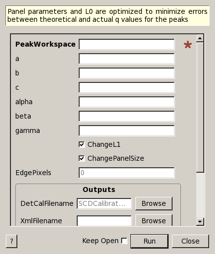
SCDCalibratePanels v1¶

SCDCalibratePanels dialog.

Table of Contents

Summary
Properties
Description
- OUTPUT workspaces and files:
After Calibration
Usage
Source

Summary ¶

Panel parameters and L0 are optimized to minimize errors between theoretical and actual q values for the peaks

Properties ¶

Name	Direction	Type	Default	Description
PeakWorkspace	InOut	PeaksWorkspace	Mandatory	Workspace of Indexed Peaks
a	Input	number	Optional	Lattice Parameter a (Leave empty to use lattice constants in peaks workspace)
b	Input	number	Optional	Lattice Parameter b (Leave empty to use lattice constants in peaks workspace)
c	Input	number	Optional	Lattice Parameter c (Leave empty to use lattice constants in peaks workspace)
alpha	Input	number	Optional	Lattice Parameter alpha in degrees (Leave empty to use lattice constants in peaks workspace)
beta	Input	number	Optional	Lattice Parameter beta in degrees (Leave empty to use lattice constants in peaks workspace)
gamma	Input	number	Optional	Lattice Parameter gamma in degrees (Leave empty to use lattice constants in peaks workspace)
ChangeL1	Input	boolean	True	Change the L1(source to sample) distance
ChangePanelSize	Input	boolean	True	Change the height and width of the detectors. Implemented only for RectangularDetectors.
EdgePixels	Input	number	0	Remove peaks that are at pixels this close to edge.
DetCalFilename	Input	string	SCDCalibrate.DetCal	Path to an ISAW-style .detcal file to save. Allowed extensions: [‘.detcal’, ‘.det_cal’]
XmlFilename	Input	string		Path to an Mantid .xml description(for LoadParameterFile) file to save. Allowed extensions: [‘.xml’]
ColFilename	Input	string	ColCalcvsTheor.nxs	Path to a NeXus file comparing calculated and theoretical column of each peak. Allowed extensions: [‘.nxs’]
RowFilename	Input	string	RowCalcvsTheor.nxs	Path to a NeXus file comparing calculated and theoretical row of each peak. Allowed extensions: [‘.nxs’]
TofFilename	Input	string	TofCalcvsTheor.nxs	Path to a NeXus file comparing calculated and theoretical TOF of each peak. Allowed extensions: [‘.nxs’]

This algorithm calibrates panels of Rectangular Detectors or packs of tubes in an instrument. The initial path, panel centers and orientations are adjusted so the error in Q positions from the theoretical Q positions is minimized. Given a set of peaks indexed by $(h_i, k_i, l_i)$ , we modify the instrument parameters, p, and then find Q in the sample frame, $\rm Q_{sample}$ that mininizes the following:

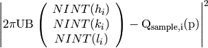
$\left\vert 2\pi \rm U \rm B \left( \begin{array}{c} NINT(h_i) \\ NINT(k_i) \\ NINT(l_i) \\ \end{array} \right) - \rm Q_{sample,i}(p) \right\vert ^2$

NINT is the nearest integer function. B is fixed from the input lattice parameters, but U is modified by CalculateUMatrix for all peaks before and after optimization. The initial path, L1, is optimized for all peaks before and after each panel or pack’s parameters are optimized. The panels and packs’ parameters are optimized in parallel. An option is available to adjust the panel widths and heights for Rectangular Detectors in a second iteration with all the other parameters fixed.

OUTPUT workspaces and files:¶

The results are saved to an ISAW-like DetCal file and optionally in an xml file that can be used with the LoadParameterFile algorithm.
There are two output workspace groups that are output when this algorithm calls the Fit algorithm.
1. Fit_Parameters: workspaces beginning with ‘params’ contains the results from fitting for each bank and for L1.
  - XShift, YShift,and ZShift are in meters.
  - XRotate, YRotate, and ZRotate are in degrees.
2. Fit_Residuals: workspaces beginning with ‘fit’ contain the differences in the calculated and theoretical Q vectors for each peak.
There are three output files that show the goodness of the calibration.
1. ColFilename contains the calculated and theoretical column for each peak. Each spectra is labeled by the bank. To plot use python script, scripts/SCD_Reduction/SCDCalibratePanelsResults.py
2. RowFilename contains the calculated and theoretical row for each peak. Each spectra is labeled by the bank. To plot use python script, scripts/SCD_Reduction/SCDCalibratePanelsResults.py
3. TofFilename contains the calculated and theoretical TOF for each peak. Each spectra is labeled by the bank.

After Calibration ¶

After calibration, you can save the workspace to Nexus (or Nexus processed) and get it back by loading in a later Mantid session. You can copy the calibration to another workspace using the same instrument by means of the CopyInstrumentParameters v1 algorithm. To do so select the workspace, which you have calibrated as the InputWorkspace and the workspace you want to copy the calibration to, the OutputWorkspace.

Usage ¶

#Calibrate peaks file and load to workspace
LoadIsawPeaks(Filename='MANDI_801.peaks', OutputWorkspace='peaks')
#TimeOffset is not stored in xml file, so use DetCal output if you need TimeOffset
SCDCalibratePanels(PeakWorkspace='peaks',DetCalFilename='mandi_801.DetCal',XmlFilename='mandi_801.xml',a=74,b=74.5,c=99.9,alpha=90,beta=90,gamma=60)
LoadEmptyInstrument(Filename=config.getInstrumentDirectory() + 'MANDI_Definition_2013_08_01.xml', OutputWorkspace='MANDI_801_event_DetCal')
CloneWorkspace(InputWorkspace='MANDI_801_event_DetCal', OutputWorkspace='MANDI_801_event_xml')
LoadParameterFile(Workspace='MANDI_801_event_xml', Filename='mandi_801.xml')
LoadIsawDetCal(InputWorkspace='MANDI_801_event_DetCal', Filename='mandi_801.DetCal')
det1 = mtd['MANDI_801_event_DetCal'].getInstrument().getDetector(327680)
det2 = mtd['MANDI_801_event_xml'].getInstrument().getDetector(327680)
if det1.getPos() == det2.getPos():
    print "matches"