UnwrapMonitorsInTOF dialog.
Table of Contents
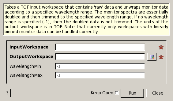
Takes a TOF input workspace that contains ‘raw’ data and unwraps monitor data according to a specified wavelength range. The monitor spectra are essentially doubled and then trimmed to the specified wavelength range. If no wavelength range is specified (-1), then the doubled data is not trimmed. The units of the output workspace is in TOF. Note that currently only workspaces with linearly binned monitor data can be handled correctly.
| Name | Direction | Type | Default | Description |
|---|---|---|---|---|
| InputWorkspace | Input | MatrixWorkspace | Mandatory | An input workspace. |
| OutputWorkspace | Output | MatrixWorkspace | Mandatory | An output workspace. |
| WavelengthMin | Input | number | -1 | A lower bound of the wavelength range. |
| WavelengthMax | Input | number | -1 | An upper bound of the wavelength range. |
This algorithm is for use with white-beam instruments with choppers. When setting two different time regimes for monitors and detectors it can occur that neutrons from the previous frame are detected by monitors further down the beam line. Note that this algorithm currently only operates well on linearly binned monitor data.
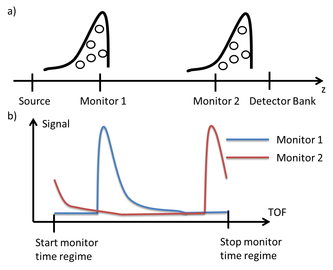
The schematic illustration below explains the situation. Two pulses are in the beam line at the same time. All monitors are operating in the same time regime. This means that while a monitor closer to the source starts detecting neutrons associated with the current frame, a monitor further down the beam line might be detecting neutrons associated with the previous frame as is depicted in illustration a) below.
This means that the measured signal for a monitor further down the beam line can be comprised of data from two sequential frames. It will be chopped up as is depicted in illustration b) below.
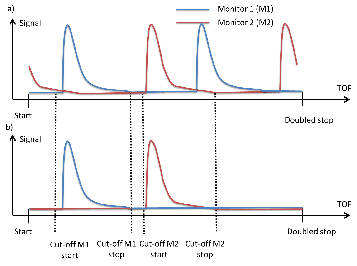
This algorithm duplicates the data and appends it to itself. This means that the TOF is essentially doubled (in the case of linear time binning). This is depicted in illustration a) below. This means that we now have data in the monitors which is not physical, i.e. some monitors seem to have measured data for certain time-of-flight values which are not accessible for the wavelength range of the apperatus and the locations of the monitors. Therefore the user can specify the wavelength range of the apperatus. This is translated into the effective time-of-flight range of each monitor and data outside of this range is set to zero. This is illustrated in image b) below.
Example - UnwrapMonitorsInTOF
import os

# Create a sample SANS2D workspace
sans2D_path = os.path.join(ConfigService.getInstrumentDirectory(),"SANS2D_Definition.xml")
workspace = LoadEmptyInstrument(sans2D_path)
workspace = Rebin(workspace, "1,10000, 100000")

# Set monitor 4  (at workspace index 3) to  [3, 2, 1, 0, 0, 0, 0, 0, 5, 4]
dataY = workspace.dataY(3)
y_values = [3, 2, 1, 0, 0, 0, 0, 0, 5, 4]
for index in range(0, 10):
    dataY[index] = y_values [index]


# Apply the UnwrapMonitorsInTOF algorithm
output_workspace = UnwrapMonitorsInTOF(InputWorkspace=workspace, WavelengthMin=5, WavelengthMax=20)

# Inspect the unwrapped data
dataY_doubled = output_workspace.dataY(3)
print("The number of bins is {0} and is expected to be 20.".format(len(dataY_doubled)))
print("The monitor 4 entries are: {0}.".format(dataY_doubled))
Output:
The number of bins is 20 and is expected to be 20.
The monitor 4 entries are: [ 0.  0.  0.  0.  0.  0.  0.  0.  5.  4.  3.  2.  1.  0.  0.  0.  0.  0.
  0.  0.].
Categories: Algorithms | CorrectionFunctions\InstrumentCorrections