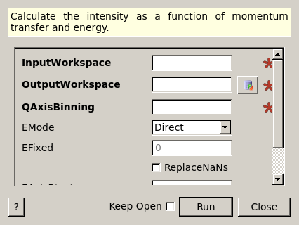
SofQWPolygon v1¶

Summary¶

Calculate the intensity as a function of momentum transfer and energy.

Properties¶

Name	Direction	Type	Default	Description
InputWorkspace	Input	MatrixWorkspace	Mandatory	Reduced data in units of energy transfer DeltaE. The workspace must contain histogram data and have common bins across all spectra.
OutputWorkspace	Output	MatrixWorkspace	Mandatory	The name to use for the q-omega workspace.
QAxisBinning	Input	dbl list	Mandatory	The bin parameters to use for the q axis (in the format used by the Rebin v1 algorithm).
EMode	Input	string	Mandatory	The energy transfer analysis mode (Direct/Indirect). Allowed values: [‘Direct’, ‘Indirect’]
EFixed	Input	number	0	The value of fixed energy: (EMode=Direct) or (EMode=Indirect) (meV). Must be set here if not available in the instrument definition.
ReplaceNaNs	Input	boolean	False	If true, all NaN values in the output workspace are replaced using the ReplaceSpecialValues algorithm.
EAxisBinning	Input	dbl list		The bin parameters to use for the E axis (optional, in the format used by the Rebin v1 algorithm).
DetectorTwoThetaRanges	Input	TableWorkspace		A table workspace use by SofQWNormalisedPolygon containing a ‘Detector ID’ column as well as ‘Min two theta’ and ‘Max two theta’ columns listing the detector’s min and max scattering angles in radians.

Description¶

Converts a 2D workspace in units of spectrum number/energy transfer to the intensity as a function of momentum transfer and energy transfer .

The rebinning is done as a weighted sum of overlapping polygons. The polygon in space is calculated from the energy bin boundaries and the detector scattering angle . The detectors (pixels) are assumed to be uniform, and characterised by a single angular width . This is calculated from the nominal of each detector; this algorithm does not utilize the DetectorTwoThetaRanges optional input property. The signal and error of the rebinned data (in space) is then the sum of the contributing pixels in each bin weighted by their fractional overlap area. Unlike the more precise SofQWNormalisedPolygon v1 algorithm, these fractional weights are not thereafter retained in the workspace produced by this algorithm.

See SofQWCentre v1 for centre-point binning. Alternatively, see SofQWNormalisedPolygon v1 for a more complex and precise (but slower) binning strategy, where the actual detector shape is calculated to obtain the input polygon.

Usage¶

Example - simple transformation of inelastic workspace:

# create sample inelastic workspace for MARI instrument containing 1 at all spectra values
ws=CreateSimulationWorkspace(Instrument='MAR',BinParams='-10,1,10')
# convert workspace into MD workspace
ws=SofQWPolygon(InputWorkspace=ws,QAxisBinning='-3,0.1,3',Emode='Direct',EFixed=12)

print("The converted X-Y values are:")
Xrow=ws.readX(59);
Yrow=ws.readY(59);
line1= " ".join('! {0:>6.2f} {1:>6.2f} '.format(Xrow[i],Yrow[i]) for i in range(0,10))
print(line1 + " !")
line2= " ".join('! {0:>6.2f} {1:>6.2f} '.format(Xrow[i],Yrow[i]) for i in range(10,20))
print(line2 + " !")
print('! {0:>6.2f} ------- !'.format(Xrow[20]))

Output:

The converted X-Y values are:
! -10.00  12.79  !  -9.00  17.63  !  -8.00  17.86  !  -7.00  18.12  !  -6.00  18.46  !  -5.00  18.69  !  -4.00  19.24  !  -3.00  19.67  !  -2.00  18.49  !  -1.00  12.00  !
!   0.00  17.08  !   1.00  22.32  !   2.00  23.26  !   3.00  24.46  !   4.00  25.96  !   5.00  21.96  !   6.00  25.10  !   7.00  33.65  !   8.00  35.54  !   9.00  43.86  !
!  10.00 ------- !

Categories: AlgorithmIndex | Inelastic\SofQW

Source¶

C++ source: SofQWPolygon.cpp (last modified: 2019-07-17)

C++ header: SofQWPolygon.h (last modified: 2018-10-05)