\(\renewcommand\AA{\unicode{x212B}}\)

MaxEnt v1¶

MaxEnt dialog.

Table of Contents

Summary
- See Also
Properties
Description
Output Workspaces
Usage
Positive Images
Complex Images
Complex Data
Increasing the number of points in the image
Adjusting the Reconstructed Data
References
Source

Summary ¶

Runs Maximum Entropy method on every spectrum of an input workspace. It currently works for the case where data and image are related by a 1D Fourier transform.

Properties ¶

Name	Direction	Type	Default	Description
InputWorkspace	Input	MatrixWorkspace	Mandatory	An input workspace.
ComplexData	Input	boolean	False	If true, the input data is assumed to be complex and the input workspace is expected to have an even number of histograms (2N). Spectrum numbers S and S+N are assumed to be the real and imaginary part of the complex signal respectively.
ComplexImage	Input	boolean	True	If true, the algorithm will use complex images for the calculations. This is the recommended option when there is no prior knowledge about the image. If the image is known to be real, this option can be set to false and the algorithm will only consider the real part for calculations.
PositiveImage	Input	boolean	False	If true, the reconstructed image is only allowed to take positive values. It can take negative values otherwise. This option defines the entropy formula that will be used for the calculations (see next section for more details).
AutoShift	Input	boolean	False	Automatically calculate and apply phase shift. Zero on the X axis is assumed to be in the first bin. If it is not, setting this property will automatically correct for this.
ResolutionFactor	Input	m	1	An integer number indicating the factor by which the number of points will be increased in the image and reconstructed data
A	Input	number	0.4	A maximum entropy constant. This algorithm was first developed for the ISIS muon group where the default 0.4 was found to give good reconstructions. In general the user will need to experiment with this value. Choosing a small value may lead to unphysical spiky reconstructions and choosing an increasingly large value the reconstruction will start to resamble that of a direct fourier transform reconstruction. However, where the data contain a zero Fourier data point with a small error the reconstruction will be insensitive to the choice of this property (and increasing so the more well determined this data point is).
ChiTargetOverN	Input	number	1	Target value of Chi-square divided by the number of data points (N)
ChiEps	Input	number	0.001	Required precision for Chi-square
DistancePenalty	Input	number	0.1	Distance penalty applied to the current image at each iteration.
MaxAngle	Input	number	0.001	Maximum degree of non-parallelism between S (the entropy) and C (chi-squared). These needs to be parallel. Chosing a smaller shouldn’t change the output. However, if you find this is the case please let the Mantid team know since this indicates that the default value of this proporty may need changing or other changes to this implementation are required.
MaxIterations	Input	m	20000	Maximum number of iterations.
AlphaChopIterations	Input	m	500	Maximum number of iterations in alpha chop.
DataLinearAdj	Input	MatrixWorkspace		Adjusts the calculated data by multiplying each value by the corresponding Y value of this workspace. The data in this workspace is complex in the same manner as complex input data.
DataConstAdj	Input	MatrixWorkspace		Adjusts the calculated data by adding to each value the corresponding Y value of this workspace. If DataLinearAdj is also specified, this addition is done after its multiplication. See equation in documentation for how DataLinearAdj and DataConstAdj are applied. The data in this workspace is complex in the same manner as complex input data.
PerSpectrumReconstruction	Input	boolean	True	Reconstruction is done independently on each spectrum. If false, all the spectra use one image and the reconstructions differ only through their adjustments. ComplexData must be set true, when this is false.
EvolChi	Output	MatrixWorkspace	Mandatory	Output workspace containing the evolution of Chi-sq.
EvolAngle	Output	MatrixWorkspace	Mandatory	Output workspace containing the evolution of non-paralellism between S and C.
ReconstructedImage	Output	MatrixWorkspace	Mandatory	The output workspace containing the reconstructed image.
ReconstructedData	Output	MatrixWorkspace	Mandatory	The output workspace containing the reconstructed data.

The maximum entropy method (MEM) is used as a signal processing technique for reconstructing images from noisy data. It selects a single image from the many images which fit the data with the same value of the statistic, \(\chi^2\). The maximum entropy method selects from this feasible set of images, the one which has minimum information (maximum entropy). More specifically, the algorithm maximizes the entropy \(S\left(x\right)\) subject to the constraint:

\[\chi^2 = \frac{1}{N'}\sum_m \frac{\left(d_m - d_m^c\right)^2}{\sigma_m^2} \leq \chi^2_{target}\]

where \(d_m\) are the experimental data, \(\sigma_m\) the associated errors, \(d_m^c\) the calculated or reconstructed data, \(\chi^2_{target}\) is value of the input algorithm property ChiTargetOverN and \(N'\) the number of measured data point. The image is a set of numbers \(\{x_0, x_1, \dots, x_{N-1}\}\) related to the measured data via a 1D Fourier transform:

\[d_m = \frac{1}{N} \sum_{j=0}^{N-1} x_j e^{i 2\pi m j / N}\]

where \(N\) is the number of image points, which can be made different from \(N'\) and is controlled by the input algorithm property ResolutionFactor, see examples further below.

Note that even for real input data the reconstructed image can be complex, which means that both the real and imaginary parts will be taken into account for the calculations. This is the default behaviour, which can be changed by setting the input property ComplexImage to False. Note that the algorithm will fail to converge if the image is complex (i.e. the data does not satisfy Friedel’s law) and this option is set to False. For this reason, it is recommended to use the default when no prior knowledge is available.

The entropy is defined on the image \(\{x_j\}\) as:

\[S = \sum_j \left[ \sqrt{x_j^2 + A^2} - x_j \sinh^{-1}\left(\frac{x_j}{A}\right) \right]\]

\[S = -\sum_j x_j \left(\log(x_j/A)-1\right)\]

where \(A\) is a constant and the formula which is used depends on the input property PositiveImage: when it is set to False the first equation will be applied, whereas the latter expression will be used if this property is set to True. The sensitive of the reconstructed image to reconstructed image will vary depending on the data. In general a smaller value would preduce a sharper image. See section 4.7 in Ref. [1] for recommended strategy to selected \(A\).

The implementation used to find the solution where the entropy is maximized subject to the constraint in \(\chi^2\) follows the approach by Skilling & Bryan [2], which is an algorithm that is not explicitly using Lagrange multiplier. Instead, they construct a subspace from a set of search directions to approach the maximum entropy solution. Initially, the image \(x\) is set to the flat background \(A\) and the search directions are constructed using the gradients of \(S\) and \(\chi^2\):

\[\mathbf{e}_1 = \left|x\right|\left(\nabla S\right)\]

\[\mathbf{e}_2 = \left|x\right|\left(\nabla \chi^2\right)\]

where \(a\left(b\right)\) stands for a componentwise multiplication between vectors \(a\) and \(b\). The algorithm next uses a quadratic approximation to determine the increment \(\delta \mathbf{x}\) that moves the image one step closer to the solution:

\[\mathbf{x} = \mathbf{x} + \delta \mathbf{x}\]

If DataLinearAdj \(l_m\) and DataConstAdj \(c_m\) are set then the reconstructed data is adjusted to

\[d_m = \frac{l_m}{N} \sum_{j=0}^{N-1} x_j e^{i 2\pi m j / N} + c_m\]

If PerSpectrumImage is set false, then chi squared is calculated for all spectra together to form a single image

\[\chi^2 = \frac{1}{N'}\sum_{m,k} \frac{\left(d_{m,k} - d_{m,k}^c\right)^2}{\sigma_{m,k}^2} \leq \chi^2_{target}\]

then the reconstructed data are calculated from this single image and the adjustments are applied for each spectrum:

\[d_{m,k} = \frac{l_{m,k}}{N} \sum_{j=0}^{N-1} x_j e^{i 2\pi m j / N} + c_{m,k}\]

Output Workspaces ¶

There are four output workspaces: ReconstructedImage and ReconstructedData contain the image and calculated data respectively, and EvolChi and EvolAngle record the algorithm’s evolution. ReconstructedData can be used to check that the calculated data approaches the experimental, measured data, and ReconstructedImage corresponds to its Fourier transform. If the input data are real they contain twice the original number of spectra, as the Fourier transform will be a complex signal in general. The real and imaginary parts are organized as follows (see Table 1): assuming your input workspace has \(M\) spectra, the real part of the reconstructed spectrum \(s\) corresponds to spectrum \(s\) in the output workspaces ReconstructedImage and ReconstructedData, while the imaginary part can be found in spectrum \(s+M\).

When the input data are complex, the input workspace is expected to have \(2M\) spectra, where real and imaginary parts of input \(s\), are arranged in spectra \((s, s+M)\) respectively. In other words, ReconstructedData and ReconstructedImage will contain \(2M\) spectra, where spectra \((s, s+M)\) correspond to the real and imaginary parts reconstructed from the input signal at \((s, s+M)\) in the input workspace (see Table 2 below).

The workspaces EvolChi and EvolAngle record the evolution of \(\chi^2\) and the angle (or non-parallelism) between \(\nabla S\) and \(\nabla \chi^2\). Note that the algorithm runs until a solution is found, and that an image is considered to be a true maximum entropy solution when the following two conditions are met simultaneously:

\[\chi^2_{Target} - \chi^2 < \epsilon_1, \qquad \frac{1}{2} \left| \frac{\nabla S}{\left|\nabla S\right|} - \frac{\nabla \chi^2}{\left|\nabla \chi^2\right|} \right| < \epsilon_2\]

While one of these conditions is not satisfied the algorithm keeps running until it reaches the maximum number of iterations. When the maximum number of iterations is reached, the last reconstructed image and its corresponding calculated data are returned, even if they do not correspond to a true maximum entropy solution satisfying the conditions above. In this way, the user can check by inspecting the output workspaces whether the algorithm was evolving towards the correct solution or not. On the other hand, the user must always check the validity of the solution by inspecting EvolChi and EvolAngle, whose values will be set to zero once the true maximum entropy solution is found.

Table 1. Output workspaces for a real input workspace with M histograms and N bins, taking J iterations.¶
Workspace	Number of histograms	Number of bins	Description
EvolChi	M	J	For spectrum \(k\) in the input workspace, evolution of \(\chi^2\) until the solution is found
EvolAngle	M	J	For spectrum \(k\) in the input workspace, evolution of the angle between \(\nabla S\) and \(\nabla \chi^2\), until the solution is found
ReconstructedImage	2M	N	For spectrum \(k\) in the input workspace, the reconstructed image is stored in spectra \(k\) (real part) and \(k+M\) (imaginary part)
ReconstructedData	2M	N	For spectrum \(k\) in the input workspace, the reconstructed data are stored in spectrum \(k\) (real part) and \(k+M\) (imaginary part). Note that although the input is real, the imaginary part is recorded for debugging purposes, it should be zero for all data points.

Table 2. Output workspaces for a complex input workspace with 2M histograms and N bins, taking J iterations.¶
Workspace	Number of histograms	Number of bins	Description
EvolChi	M	J	For spectrum \((k, k+M)\) in the input workspace, evolution of \(\chi^2\) until the solution is found
EvolAngle	M	J	For spectrum \((k, k+M)\) in the input workspace, evolution of the angle between \(\nabla S\) and \(\nabla \chi^2\), until the solution is found
ReconstructedImage	2M	\(N\)	For spectrum \((k, k+M)\) in the input workspace, the reconstructed image is stored in spectra \(k\) (real part) and \(k+M\) (imaginary part)
ReconstructedData	2M	\(N\)	For spectrum \((k, k+M)\) in the input workspace, the reconstructed data are stored in spectra \(k\) (real part) and \(k+M\) (imaginary part)

Usage ¶

Some of the usage examples use usage data files.

Note

To run these usage examples please first download the usage data, and add these to your path. In Mantid this is done using Manage User Directories.

Example - Reconstruct Fourier coefficients

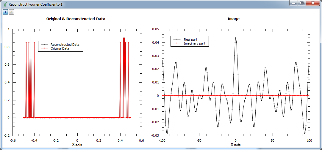
In the example below, a workspace containing five Fourier coefficients is created and used as input to MaxEnt v1. In the figure we show the original and reconstructed data (left), and the reconstructed image, i.e. Fourier transform (right).

# Create an empty workspace
X = []
Y = []
E = []
N = 200
for i in range(0,N):
    x = ((i-N/2) *1./N)
    X.append(x)
    Y.append(0)
    E.append(0.001)

# Fill in five Fourier coefficients
# The input signal must be symmetric to get a real image
Y[5] = Y[195] = 0.85
Y[10] = Y[190] = 0.85
Y[20] = Y[180] = 0.85
Y[12] = Y[188] = 0.90
Y[14] = Y[186] = 0.90
CreateWorkspace(OutputWorkspace='inputws',DataX=X,DataY=Y,DataE=E,NSpec=1)
evolChi, evolAngle, image, data = MaxEnt(InputWorkspace='inputws', A=0.0001)

print("First  reconstructed coefficient: {:.3f}".format(data.readY(0)[5]))
print("Second reconstructed coefficient: {:.3f}".format(data.readY(0)[10]))
print("Third  reconstructed coefficient: {:.3f}".format(data.readY(0)[20]))
print("Fourth reconstructed coefficient: {:.3f}".format(data.readY(0)[12]))
print("Fifth  reconstructed coefficient: {:.3f}".format(data.readY(0)[14]))
print("Number of iterations: "+str( len(evolAngle.readX(0))))

Output:

First  reconstructed coefficient: 0.847
Second reconstructed coefficient: 0.846
Third  reconstructed coefficient: 0.846
Fourth reconstructed coefficient: 0.896
Fifth  reconstructed coefficient: 0.896
Number of iterations: ...

../_images/MaxEntFourierCoefficients.png

Example - Reconstruct a real muon dataset

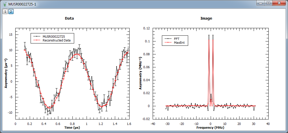
In this example, MaxEnt v1 is run on a pre-analyzed muon dataset. The corresponding figure shows the original and reconstructed data (left), and the real part of the image obtained with MaxEnt v1 and FFT v1 (right).

Load(Filename=r'MUSR00022725.nxs', OutputWorkspace='MUSR00022725')
CropWorkspace(InputWorkspace='MUSR00022725', OutputWorkspace='MUSR00022725', XMin=0.11, XMax=1.6, EndWorkspaceIndex=0)
RemoveExpDecay(InputWorkspace='MUSR00022725', OutputWorkspace='MUSR00022725')
Rebin(InputWorkspace='MUSR00022725', OutputWorkspace='MUSR00022725', Params='0.016')
evolChi, evolAngle, image, data = MaxEnt(InputWorkspace='MUSR00022725', A=0.005)
# Compare MaxEnt to FFT
imageFFT = FFT(InputWorkspace='MUSR00022725')

print("Image at {:.3f}: {:.3f}".format(image.readX(0)[44], image.readY(0)[44]))
print("Image at {:.3f}: {:.3f}".format(image.readX(0)[46], image.readY(0)[46]))
print("Image at {:.3f}: {:.3f}".format(image.readX(0)[48], image.readY(0)[48]))
# check background is not nosiy
def getInt(originalX,originalY,xMin,xMax):
   import numpy as np
   yData=[]
   xData=[]
   for j in range(0,len(originalX)):
       if originalX[j]>xMin and originalX[j]<xMax:
           yData.append(originalY[j]**2)
           xData.append(originalX[j])
   return np.trapz(x=xData,y=np.sqrt(yData))
# Do not change these numbers - they test if noise has been added to the alg
print("Negative background {:.6f}".format(getInt(image.readX(0), image.readY(0),-30,-2 )))
print("Positive background {:.6f}".format(getInt(image.readX(0), image.readY(0),2,30 )))
print ("Number of iterations: "+str( len(evolAngle.readX(0))))

Output:

Image at -1.359: 0.100
Image at 0.000: 0.009
Image at 1.359: 0.100
Negative background 0.006431
Positive background 0.006431
Number of iterations: ...

Next, MaxEnt v1 is run on a different muon dataset. The figure shows the original and reconstructed data (left), the real part of the image (middle) and its imaginary part (right).

Load(Filename=r'EMU00020884.nxs', OutputWorkspace='EMU00020884')
CropWorkspace(InputWorkspace='EMU00020884', OutputWorkspace='EMU00020884', XMin=0.17, XMax=4.5, EndWorkspaceIndex=0)
RemoveExpDecay(InputWorkspace='EMU00020884', OutputWorkspace='EMU00020884')
Rebin(InputWorkspace='EMU00020884', OutputWorkspace='EMU00020884', Params='0.016')
evolChi, evolAngle, image, data = MaxEnt(InputWorkspace='EMU00020884', A=0.0001, MaxIterations=2500, ChiTargetOverN=300.0/270.0)
# Compare MaxEnt to FFT
imageFFT = FFT(InputWorkspace='EMU00020884')

print("Image (real part) at {:.3f}: {:.3f}".format(image.readX(0)[129], image.readY(0)[129]))
print("Image (real part) at  {:.3f}:  {:.3f}".format(image.readX(0)[135], image.readY(0)[135]))
print("Image (real part) at  {:.3f}: {:.3f}".format(image.readX(0)[141], image.readY(0)[141]))
print("Image (imaginary part) at {:.3f}: {:.3f}".format(image.readX(1)[129], image.readY(1)[129]))
print("Image (imaginary part) at  {:.3f}:  {:.3f}".format(image.readX(1)[135], image.readY(1)[135]))
print("Image (imaginary part) at  {:.3f}:  {:.3f}".format(image.readX(1)[141], image.readY(1)[141]))
print ("Number of iterations: "+str( len(evolAngle.readX(0))))

Output:

Image (real part) at -1.389: -0.063
Image (real part) at  0.000:  0.035
Image (real part) at  1.389: -0.063
Image (imaginary part) at -1.389: -0.277
Image (imaginary part) at  0.000:  0.000
Image (imaginary part) at  1.389:  0.277
Number of iterations: ...

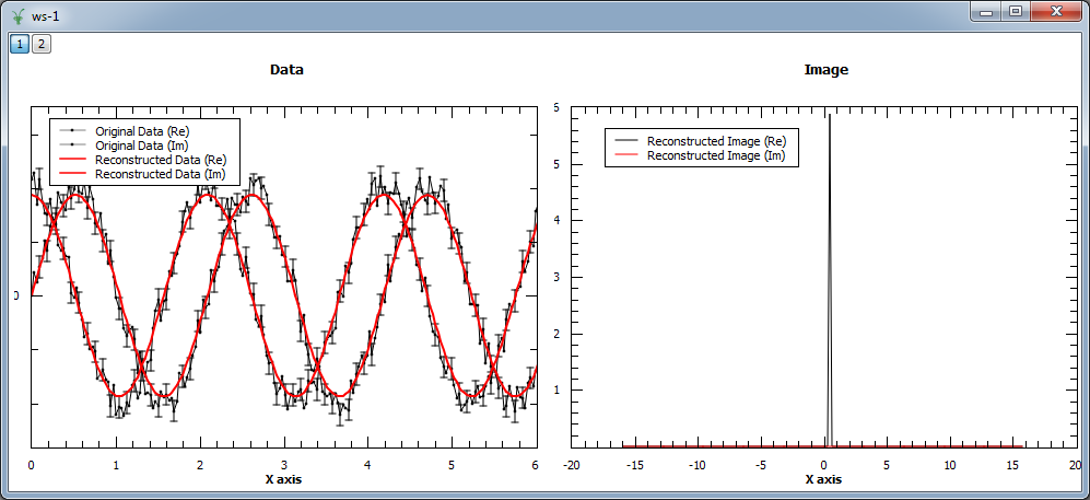
Finally, we show an example where a complex signal is analyzed. In this case, the input workspace contains two spectra corresponding to the real and imaginary part of the same signal. The figure shows the original and reconstructed data (left), and the reconstructed image (right).

from math import pi, sin, cos
from random import random, seed
seed(0)
# Create a test workspace
X = []
YRe = []
YIm = []
E = []
N = 200
w = 3
for i in range(0,N):
    x = 2*pi*i/N
    X.append(x)
    YRe.append(cos(w*x)+(random()-0.5)*0.3)
    YIm.append(sin(w*x)+(random()-0.5)*0.3)
    E.append(0.1)
CreateWorkspace(OutputWorkspace='ws',DataX=X+X,DataY=YRe+YIm,DataE=E+E,NSpec=2)
evolChi, evolAngle, image, data = MaxEnt(InputWorkspace='ws', ComplexData=True, A=0.001)

print("Image (real part) at {:.3f}: {:.3f}".format(image.readX(0)[102], image.readY(0)[102]))
print("Image (real part) at {:.3f}: {:.3f}".format(image.readX(0)[103], image.readY(0)[103]))
print("Image (real part) at {:.3f}: {:.3f}".format(image.readX(0)[104], image.readY(0)[104]))
print ("Number of iterations: "+str( len(evolAngle.readX(0))))

Output:

Image (real part) at 0.318: 0.000
Image (real part) at 0.477: 5.862
Image (real part) at 0.637: 0.000
Number of iterations: ...

Positive Images ¶

The algorithm allows users to restrict the reconstructed image to positive values only. This behaviour can be selected by setting the input property PositiveImage to true. In this case, the entropy is defined by the expression:

\[S = -\sum_j x_j \left(\log(x_j/A)-1\right)\]

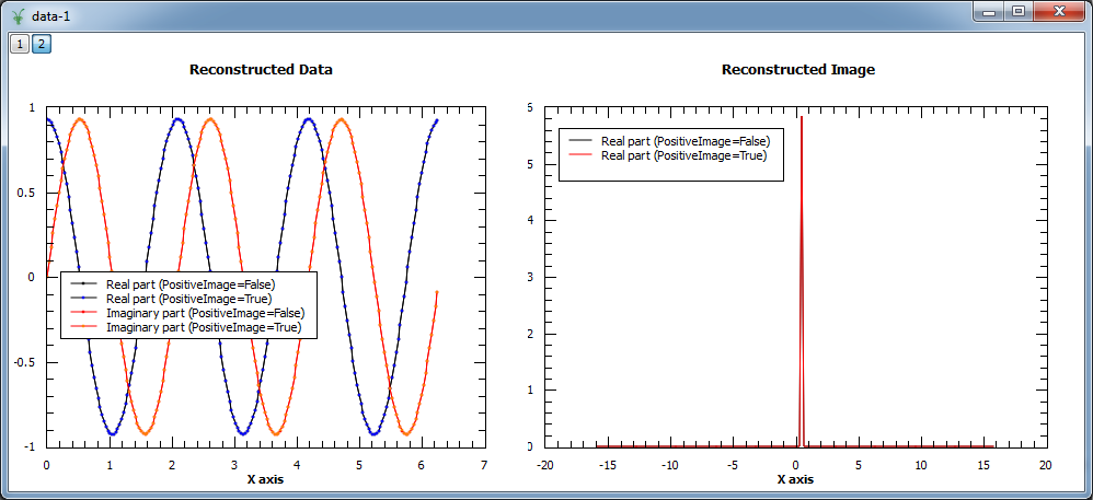
In addition, the algorithm explicitly protects against negative values by setting those to a fraction of the maximum entropy constant A. In the example below both modes are compared. As the input is a complex signal with expected Fourier transform \(F(\omega) = \delta\left(\omega-\omega_0\right)\), i.e. positive, both modes should produce the same results (note that the maximum entropy constant A typically needs to be set to smaller values for positive image in order to obtain smooth results).

from math import pi, sin, cos
from random import random, seed
seed(0)
# Create a test workspace
X = []
YRe = []
YIm = []
E = []
N = 200
w = 3
for i in range(0,N):
    x = 2*pi*i/N
    X.append(x)
    YRe.append(cos(w*x)+(random()-0.5)*0.3)
    YIm.append(sin(w*x)+(random()-0.5)*0.3)
    E.append(0.1)
CreateWorkspace(OutputWorkspace='ws',DataX=X+X,DataY=YRe+YIm,DataE=E+E,NSpec=2)
evolChi, evolAngle, image, data = MaxEnt(InputWorkspace='ws', ComplexData=True, A=0.001, PositiveImage=False)
evolChiP, evolAngleP, imageP, dataP = MaxEnt(InputWorkspace='ws', ComplexData=True, A=0.001, PositiveImage=True)

print("Image at {:.3f}: {:.3f} (PositiveImage=False), {:.3f} (PositiveImage=True)".format(image.readX(0)[102], image.readY(0)[102], imageP.readY(0)[102]))
print("Image at {:.3f}: {:.3f} (PositiveImage=False), {:.3f} (PositiveImage=True)".format(image.readX(0)[103], image.readY(0)[103], imageP.readY(0)[103]))
print("Image at {:.3f}: {:.3f} (PositiveImage=False), {:.3f} (PositiveImage=True)".format(image.readX(0)[104], image.readY(0)[104], imageP.readY(0)[102]))
print ("Number of iterations: "+str( len(evolAngle.readX(0))))
print ("Number of iterations: "+str( len(evolAngleP.readX(0))))

Output:

Image at 0.318: 0.000 (PositiveImage=False), 0.000 (PositiveImage=True)
Image at 0.477: 5.862 (PositiveImage=False), 5.913 (PositiveImage=True)
Image at 0.637: 0.000 (PositiveImage=False), 0.000 (PositiveImage=True)
Number of iterations: ...
Number of iterations: ...

Complex Images ¶

By default the input property ComplexImage is set to True and the algorithm will assume complex images for the calculations. This means that the set of numbers \(\{x_j\}\) that form the image will have a real and an imaginary part, and both components will be considered to evaluate the entropy, \(S\left(x_j\right)\), and its derivative, \(\nabla S\left(x_j\right)\). This effectively means splitting the entropy (the same applies to its derivative) in two terms, \(S\left(x_j\right) = \left[S\left(x_j^{re}\right), S\left(x_j^{im}\right)\right]\), where the first one refers to the real part of the entropy and the second one to the imaginary part. This is the recommended option when no prior knowledge about the image is available, as trying to reconstruct images that are inherently complex discarding the imaginary part will prevent the algorithm from converging. If the image is known to be real this property can be safely set to False.

Complex Data ¶

If the input property ComplexData is set to True, the algorithm will assume complex data for the calculations with all the real parts listed before all the imaginary parts. This means that if you have workspaces where the imaginary part immediately follow the real part, such workspaces cannot be combined by using the AppendSpectra v1 algorithm because the resulting output will not order the real and imaginary parts corrected as needed for this algorithm. The following usage example shows how to combine two workspaces with complex data.

from math import pi, sin, cos
from random import random, seed
seed(0)
# Create complex data for a workspace
X = []
YRe = []
YIm = []
E = []
N = 200
w = 3
for i in range(0,N):
    x = 2*pi*i/N
    X.append(x)
    YRe.append(cos(w*x)+(random()-0.5)*0.3)
    YIm.append(sin(w*x)+(random()-0.5)*0.3)
    E.append(0.1)

seed(0)
# Create complex data for a second workspace
X2 = []
YRe2 = []
YIm2 = []
E2 = []
N2 = 200
w2 = 4
for i in range(0,N2):
    x = 2*pi*i/N2
    X2.append(x)
    YRe2.append(cos(w2*x)+(random()-0.5)*0.3)
    YIm2.append(sin(w2*x)+(random()-0.5)*0.3)
    E2.append(0.5)

# Create two workspaces of one spectrum each
CreateWorkspace(OutputWorkspace='ws1',DataX=X+X,DataY=YRe+YIm,DataE=E+E,NSpec=2)
evolChiP, evolAngleP, imageP, dataP = MaxEnt(InputWorkspace='ws1', ComplexData=True, A=0.001, PositiveImage=True)

print ("Number of iterations dataset1 separate: "+str( len(evolAngleP.readX(0))))

CreateWorkspace(OutputWorkspace='ws2',DataX=X2+X2,DataY=YRe2+YIm2,DataE=E2+E2,NSpec=2)
evolChiP2, evolAngleP2, imageP2, dataP2 = MaxEnt(InputWorkspace='ws2', ComplexData=True, A=0.001, PositiveImage=True)

print ("Number of iterations dataset2 separate: "+str( len(evolAngleP2.readX(0))))

# Combine the two workspaces
CreateWorkspace(OutputWorkspace='wsCombined',DataX=X+X2+X+X2,DataY=YRe+YRe2+YIm+YIm2,DataE=E+E2+E+E2,NSpec=4)
evolChiC, evolAngleC, imageC, dataC = MaxEnt(InputWorkspace='wsCombined', ComplexData=True, A=0.001, PositiveImage=True)

print ("Number of iterations dataset1 combined: "+str( len(evolAngleC.readX(0))))
print ("Number of iterations dataset2 combined: "+str( len(evolAngleC.readX(1))))

Output:

Number of iterations dataset1 separate: ...
Number of iterations dataset2 separate: ...
Number of iterations dataset1 combined: ...
Number of iterations dataset2 combined: ...

Increasing the number of points in the image ¶

The algorithm has an input property, ResolutionFactor, that allows to increase the number of points in the reconstructed image. This is at present done by extending the range (and therefore the number of points) in the reconstructed data. The number of reconstructed points can be increased by any integer factor, but note that this will slow down the algorithm and you may need to increase the number of maxent iterations so that the algorithm is able to converge to a solution.

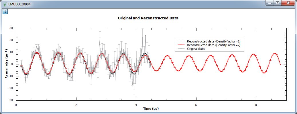
An example script where the density of points is increased by a factor of 2 can be found below. Note that when a factor of 2 is used, the reconstructed data is twice the size of the original (experimental) data. Also shown is how ChiTargetOverN property may be varied away from the default 1.0; the dataset contains 270 data points and here set to be slightly higher at 300/270.

Load(Filename=r'EMU00020884.nxs', OutputWorkspace='ws')
CropWorkspace(InputWorkspace='ws', OutputWorkspace='ws', XMin=0.17, XMax=4.5, EndWorkspaceIndex=0)
ws = RemoveExpDecay(InputWorkspace='ws')
ws = Rebin(InputWorkspace='ws', Params='0.016')
evolChi1, evolAngle1, image1, data1 = MaxEnt(InputWorkspace='ws', A=0.0001, MaxIterations=2500, ResolutionFactor=1, ChiTargetOverN=300.0/270.0)
evolChi2, evolAngle2, image2, data2 = MaxEnt(InputWorkspace='ws', A=0.0001, MaxIterations=5000, ResolutionFactor=2, ChiTargetOverN=300.0/270.0)

print("Image at {:.3f}: {:.3f} (ResolutionFactor=1)".format(image1.readX(0)[135], image1.readY(0)[135]))
print("Image at {:.3f}: {:.3f} (ResolutionFactor=2)".format(image2.readX(0)[270], image2.readY(0)[270]))
print ("Number of iterations: "+str( len(evolAngle1.readX(0))))
print ("Number of iterations: "+str( len(evolAngle2.readX(0))))

Output:

Image at 0.000: 0.035 (ResolutionFactor=1)
Image at 0.000: 0.068 (ResolutionFactor=2)
Number of iterations: ...
Number of iterations: ...

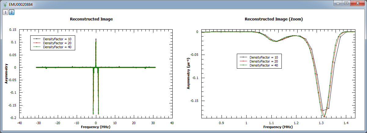
In the next example, we increased the density of points by factors of 10, 20 and 40. We show the reconstructed image (left) and a zoom into the region \(0.82 < x < 1.44\) and \(-0.187 < y < 0.004\).

Load(Filename=r'EMU00020884.nxs', OutputWorkspace='ws')
CropWorkspace(InputWorkspace='ws', OutputWorkspace='ws', XMin=0.17, XMax=4.5, EndWorkspaceIndex=0)
ws = RemoveExpDecay(InputWorkspace='ws')
ws = Rebin(InputWorkspace='ws', Params='0.016')
evolChi1, evolAngle1, image1, data1 = MaxEnt(InputWorkspace='ws', A=0.0001, MaxIterations=2500, ResolutionFactor=1)
evolChi10, evolAngle10, image10, data10 = MaxEnt(InputWorkspace='ws', A=0.0001, MaxIterations=25000, ResolutionFactor=10)
evolChi20, evolAngle20, image20, data20 = MaxEnt(InputWorkspace='ws', A=0.0001, MaxIterations=50000, ResolutionFactor=20)
evolChi40, evolAngle40, image40, data40 = MaxEnt(InputWorkspace='ws', A=0.0001, MaxIterations=75000, ResolutionFactor=40)

print ("Number of iterations: "+str( len(evolAngle1.readX(0))))
print ("Number of iterations: "+str( len(evolAngle10.readX(0))))
print ("Number of iterations: "+str( len(evolAngle20.readX(0))))
print ("Number of iterations: "+str( len(evolAngle40.readX(0))))

Output:

Number of iterations: ...
Number of iterations: ...
Number of iterations: ...
Number of iterations: ...

Adjusting the Reconstructed Data ¶

The reconstructed data can be adjusted by multiplying by the DataLinearAdj property and then adding the DataConstAdj property. Each of these properties is a workspace with complex Y values, just like complex input workspaces. Each Y value is then applied to the corresponding Y values in the reconstructed data at each iteration.

These usage examples merely demonstrate how to use the adjustments and are not realistic use cases.

from math import pi, sin, cos
from random import random, seed

# Construct workspace (cosine + noise) over 3 spectra
X = []
Y = []
E = []
N = 200
w = 3
for s in range(0,3):
    seed(0)
    for i in range(0,N):
        x = 2*pi*i/N
        X.append(x)
        Y.append(cos(w*x)+(random()-0.5)*0.3)
        E.append(0.2)

CreateWorkspace(OutputWorkspace='inputws',DataX=X,DataY=Y,DataE=E,NSpec=3)

# Construct linear adjustment workspace (real = 1, imaginary linear)
# no adjustment on first spectrum, double adjustment on third spectrum.
Zeroes = []
Ylin = []
Magnitude = - 0.1
# Real values
for s in range(0,3):
    for i in range(0,N):
        Ylin.append(1.0)
        Zeroes.append(0)

# Imaginary values
for s in range(0,3):
    for i in range(0,N):
        X.append(X[i])
        Ylin.append(s*Magnitude*X[i])
        Zeroes.append(0)

CreateWorkspace(OutputWorkspace='linadj', DataX=X, DataY=Ylin, DataE=Zeroes, NSpec=6)

# Construct constant adjustment workspace (real = 0, imaginary linear)
# no adjustment on first spectrum, double adjustment on third spectrum.
Yconst = []
Magnitude = 0.2
# Real values
for s in range(0,3):
    for i in range(0,N):
        Yconst.append(0)

# Imaginary values
for s in range(0,3):
    for i in range(0,N):
        Yconst.append(s*Magnitude*X[i])

CreateWorkspace(OutputWorkspace='constadj',DataX=X, DataY=Yconst, DataE=Zeroes, NSpec=6)

evolChi, evolAngle, image, data = MaxEnt(InputWorkspace='inputws', DataLinearAdj='linadj', DataConstAdj='constadj',A=0.001)

print("Reconstruction at 05 of first spectrum: {:.3f}".format(data.readY(0)[5]))
print("Reconstruction at 10 of first spectrum: {:.3f}".format(data.readY(0)[10]))
print("Reconstruction at 15 of first spectrum: {:.3f}".format(data.readY(0)[15]))
print("Reconstruction at 05 of third spectrum: {:.3f}".format(data.readY(2)[5]))
print("Reconstruction at 10 of third spectrum: {:.3f}".format(data.readY(2)[10]))
print("Reconstruction at 15 of third spectrum: {:.3f}".format(data.readY(2)[15]))
print("Number of iterations of first spectrum: "+str( len(evolAngle.readX(0))))
print("Number of iterations of second spectrum: "+str( len(evolAngle.readX(1))))
print("Number of iterations of third spectrum: "+str( len(evolAngle.readX(2))))

Output:

Reconstruction at 05 of first spectrum: 0.657
Reconstruction at 10 of first spectrum: 0.433
Reconstruction at 15 of first spectrum: 0.115
Reconstruction at 05 of third spectrum: 0.522
Reconstruction at 10 of third spectrum: 0.485
Reconstruction at 15 of third spectrum: -0.019
Number of iterations of first spectrum: 5
Number of iterations of second spectrum: 37
Number of iterations of third spectrum: 70

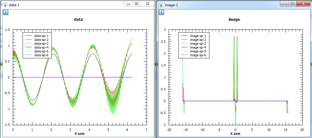
The first plot shows the reconstructed data and the second plot the corresponding image. The first three spectra plotted are the real parts of the 3 spectra and the other three spectra are the imaginary parts.

This can also be done with the spectra of the data effectively concatenated and converted into a single image. The reconstructed data is then obtained by converting the image back to data, copying for each spectrum and applying the adjustments.

This is done by setting the PerSpectrumImage property to false.

from math import pi, sin, cos
from random import random, seed

# Construct workspace (real cosine + complex noise) over 3 spectra
X = []
Y = []
E = []
N = 200
w = 3
for s in range(0,3):
   # Real values
   seed(0)
   for i in range(0,N):
     x = 2*pi*i/N
     X.append(x)
     Y.append(cos(w*x)+(random()-0.5)*0.3)
     E.append(0.27)

for s in range(0,3):
   # Imaginary values
   for i in range(0,N):
     x = 2*pi*i/N
     X.append(x)
     Y.append((random()-0.5)*0.3)
     E.append(0.27)

CreateWorkspace(OutputWorkspace='inputws',DataX=X,DataY=Y,DataE=E,NSpec=6)

# Construct linear adjustment workspace (real = 1, imaginary linear)
# no adjustment on first spectrum, double adjustment on third spectrum.
Zeroes = []
Xlin = []
Ylin = []
Magnitude = - 0.14
for s in range(0,3):
   # Real values
   for i in range(0,N):
      Xlin.append(X[i])
      Ylin.append(1.0)
      Zeroes.append(0)

for s in range(0,3):
   # Imaginary values
   for i in range(0,N):
      Xlin.append(X[i])
      Ylin.append(s*Magnitude*X[i])
      Zeroes.append(0)

CreateWorkspace(OutputWorkspace='linadj', DataX=Xlin, DataY=Ylin, DataE=Zeroes, NSpec=6)

# Construct constant adjustment workspace (real = 0, imaginary linear)
# no adjustment on first spectrum, double adjustment on third spectrum.
Yconst = []
Magnitude = -0.05
# Real values
for s in range(0,3):
    for i in range(0,N):
       Yconst.append(0)

# Imaginary values
for s in range(0,3):
    for i in range(0,N):
        Yconst.append(s*Magnitude*X[i])


CreateWorkspace(OutputWorkspace='constadj',DataX=Xlin, DataY=Yconst, DataE=Zeroes, NSpec=6)

evolChi, evolAngle, image, data = MaxEnt(InputWorkspace='inputws', ComplexData=True, DataLinearAdj='linadj', DataConstAdj='constadj',A=0.001, PerSpectrumReconstruction=False)

print("Reconstruction at 05 of first spectrum: {:.3f}".format(data.readY(0)[5]))
print("Reconstruction at 10 of first spectrum: {:.3f}".format(data.readY(0)[10]))
print("Reconstruction at 15 of first spectrum: {:.3f}".format(data.readY(0)[15]))
print("Reconstruction at 05 of third spectrum: {:.3f}".format(data.readY(2)[5]))
print("Reconstruction at 10 of third spectrum: {:.3f}".format(data.readY(2)[10]))
print("Reconstruction at 15 of third spectrum: {:.3f}".format(data.readY(2)[15]))

Output:

Reconstruction at 05 of first spectrum: 0.679
Reconstruction at 10 of first spectrum: 0.470
Reconstruction at 15 of first spectrum: 0.158
Reconstruction at 05 of third spectrum: 0.687
Reconstruction at 10 of third spectrum: 0.481
Reconstruction at 15 of third spectrum: 0.163

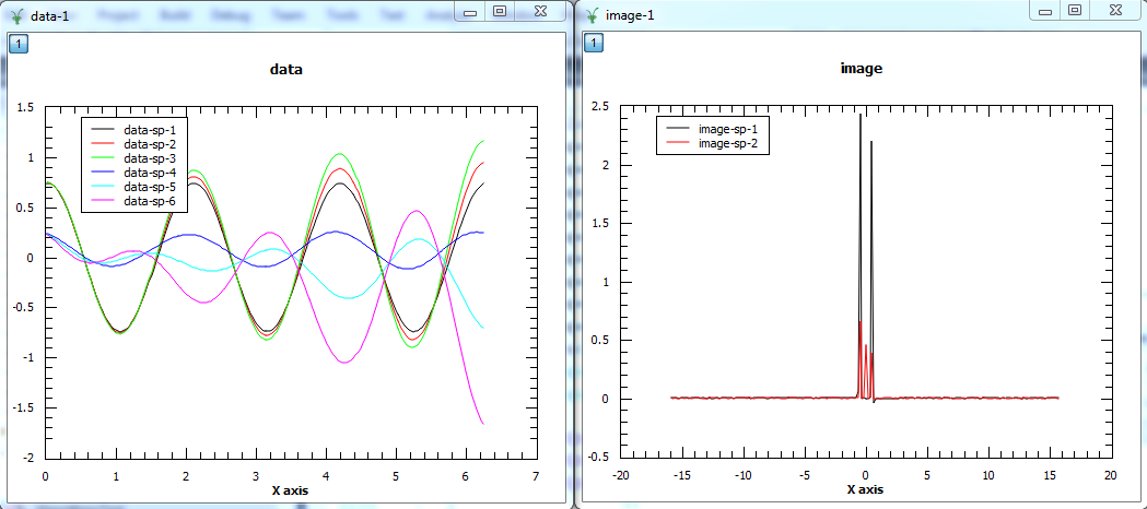
The first plot shows the reconstructed data and the second plot the corresponding image. In the data, the first three spectra plotted are the real parts of the 3 spectra and the other three spectra are the imaginary parts. In the image, the first spectrum is the real part and the second spectrum is the imaginary part.

References ¶

[1] Anders Johannes Markvardsen, (2000). Polarised neutron diffraction measurements of PrBa2Cu3O6+x and the Bayesian statistical analysis of such data. DPhil. University of Oxford (http://ora.ox.ac.uk/objects/uuid:bef0c991-4e1c-4b07-952a-a0fe7e4943f7)

[2] Skilling & Bryan, (1984). Maximum entropy image reconstruction: general algorithm. Mon. Not. R. astr. Soc. 211, 111-124.

Categories: AlgorithmIndex | Arithmetic\FFT

Source ¶

C++ header: MaxEnt.h (last modified: 2020-10-16)

C++ source: MaxEnt.cpp (last modified: 2020-10-16)

MaxEnt v1¶

Summary ¶

See Also ¶

Properties ¶

Description ¶

Output Workspaces ¶

Usage ¶

Positive Images ¶

Complex Images ¶

Complex Data ¶

Increasing the number of points in the image ¶

Adjusting the Reconstructed Data ¶

References ¶

Source ¶