\(\renewcommand\AA{\unicode{x212B}}\)

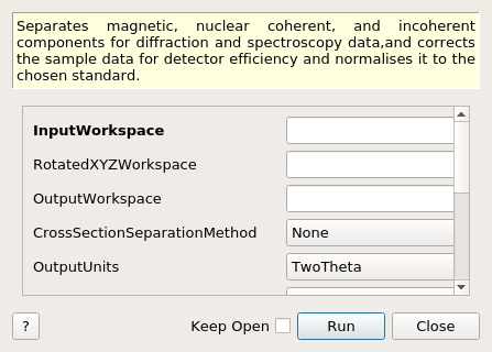
D7AbsoluteCrossSections v1¶

D7AbsoluteCrossSections dialog.

Table of Contents

Summary
- See Also
Properties
Description
Usage
References
Source

Summary ¶

Separates magnetic, nuclear coherent, and incoherent components for diffraction and spectroscopy data,and corrects the sample data for detector efficiency and normalises it to the chosen standard.

Properties ¶

Name	Direction	Type	Default	Description
InputWorkspace	Input	WorkspaceGroup	Mandatory	The input workspace with spin-flip and non-spin-flip data.
RotatedXYZWorkspace	Input	WorkspaceGroup		The workspace used in 10p method when data is taken as two XYZ measurements rotated by 45 degress.
OutputWorkspace	Output	WorkspaceGroup		The output workspace.
CrossSectionSeparationMethod	Input	string	None	What type of cross-section separation to perform. Allowed values: [‘None’, ‘Uniaxial’, ‘XYZ’, ‘10p’]
OutputUnits	Input	string	TwoTheta	The choice to display the output either as a function of detector twoTheta, or the momentum exchange. Allowed values: [‘TwoTheta’, ‘Q’]
NormalisationMethod	Input	string	None	Method to correct detector efficiency and normalise data. Allowed values: [‘None’, ‘Vanadium’, ‘Incoherent’, ‘Paramagnetic’]
OutputTreatment	Input	string	Individual	Which treatment of the provided scan should be used to create output. Allowed values: [‘Individual’, ‘Merge’]
SampleAndEnvironmentProperties	Input	Dictionary	dict()	Dictionary for the information about sample and its environment.
ScatteringAngleBinSize	Input	number	0.5	Scattering angle bin size in degrees used for expressing scan data on a single TwoTheta axis.
VanadiumInputWorkspace	Input	WorkspaceGroup		The name of the vanadium workspace.
AbsoluteUnitsNormalisation	Input	boolean	True	Whether or not express the output in absolute units.
ClearCache	Input	boolean	True	Whether or not to delete intermediate workspaces.

This is the algorithm that performs cross-section separation and allows for sample data normalisation to absolute scale. The cross-section separation provides information about magnetic, nuclear coherent, and spin-incoherent contributions to the measured cross-section. The absolute scale normalisation uses either the output from cross-section separation or a vanadium reference sample for polarised diffraction and spectroscopy data measured by D7 instrument at the ILL.

Three types of cross-section separation are supported: Uniaxial, XYZ, and 10p, for which 2, 6, and 10 distributions with spin-flip and non-spin-flip cross-sections are required. The expected input is a workspace group containing spin-flip and non-spin-flip cross-sections, with the following order of axis directions: Z, Y, X, X-Y, X+Y. This step can be skipped by setting CrossSectionSeparationMethod parameter to ‘None’.

Three ways of sample data normalisation are supported: Vanadium, Paramagnetic, and Incoherent, for which either the output from vanadium data reduction, or from the cross-section separation (magnetic and spin-incoherent respectively) is used. This step can also be skipped by setting NormalisationMethod parameter to ‘None’.

This algorithm is indended to be invoked on sample data that is fully corrected and needs to be normalised to the absolute scale.

SampleAndEnvironmentProperties ¶

This property is a dictionary containing all of the information about the sample and its environment, in the same fashion as in PolDiffILLReduction. This information is used for proper normalisation of the given sample.

The following keys need to be defined:

SampleMass
FormulaUnits
FormulaUnitMass
SampleSpin if the NormalisationMethod is set to Paramagnetic
IncoherentCrossSection if the NormalisationMethod is set to Incoherent and AbsoluteUnitsNormalisation is True

Cross-section separation method ¶

Below are presented formulae used to separate magnetic (M), nuclear coherent (N), and spin-incoherent (I) cross-sections using spin-flip \(\left(\frac{d\sigma}{d\Omega}\right)_{\text{sf}}\) and non-spin-flip \(\left(\frac{d\sigma}{d\Omega}\right)_{\text{nsf}}\) cross-sections from the provided input WorkspaceGroup.

Uniaxial

At least two separate measurements along the same axis with opposite spin orientations are needed for this method to work. Usually, the measured axis is the ‘Z’ axis that is colinear with the beam axis, thus the spin-flip and non-spin-flip cross-sections are measured along the longitudinal axis. This method does not allow for separation of magnetic cross-section.

\[ \begin{align}\begin{aligned}N = 2 \cdot \left(\frac{\text{d}\sigma_{z}}{\text{d}\Omega}\right)_{\text{nsf}} - \left(\frac{\text{d}\sigma_{z}}{\text{d}\Omega}\right)_{\text{sf}}\\I = 2 \cdot \left(\frac{\text{d}\sigma_{z}}{\text{d}\Omega}\right)_{\text{sf}} - \left(\frac{\text{d}\sigma_{z}}{\text{d}\Omega}\right)_{\text{nsf}}\end{aligned}\end{align} \]

In this case, the magnetic cross-section cannot be separated from data.

This method is an expansion of the Uniaxial method, that requires measurements of spin-flip and non-spin-flip cross-sections along three orthogonal axes. This method allows for separation of magnetic cross-section from nuclear coherent and spin-incoherent.

\[ \begin{align}\begin{aligned}T &= \frac{1}{3} \cdot \left( \left(\frac{\text{d}\sigma_{x}}{\text{d}\Omega}\right)_{\text{nsf}} + \left(\frac{\text{d}\sigma_{y}}{\text{d}\Omega}\right)_{\text{nsf}} + \left(\frac{\text{d}\sigma_{z}}{\text{d}\Omega}\right)_{\text{nsf}} + \left(\frac{\text{d}\sigma_{x}}{\text{d}\Omega}\right)_{\text{sf}} + \left(\frac{\text{d}\sigma_{y}}{\text{d}\Omega}\right)_{\text{sf}} + \left(\frac{\text{d}\sigma_{z}}{\text{d}\Omega}\right)_{\text{sf}} \right)\\M_{\text{nsf}} &= 2 \cdot \left(2 \cdot \left(\frac{\text{d}\sigma_{z}}{\text{d}\Omega}\right)_{\text{nsf}} - \left(\frac{d\sigma_{x}}{\text{d}\Omega}\right)_{\text{nsf}} - \left(\frac{\text{d}\sigma_{y}}{\text{d}\Omega}\right)_{\text{nsf}} \right)\\M_{\text{sf}} &= 2 \cdot \left(\left(\frac{d\sigma_{x}}{\text{d}\Omega}\right)_{\text{sf}} + \left(\frac{\text{d}\sigma_{y}}{\text{d}\Omega}\right)_{\text{sf}} -2 \cdot \left(\frac{\text{d}\sigma_{z}}{\text{d}\Omega}\right)_{\text{sf}} \right)\\M_{\text{av}} &= \frac{1}{2} \cdot \left( M_{\text{nsf}} + M_{\text{sf}} \right)\\N &= \frac{1}{6} \cdot \left(2 \cdot \left( \left(\frac{\text{d}\sigma_{x}}{\text{d}\Omega}\right)_{\text{nsf}} + \left(\frac{\text{d}\sigma_{y}}{\text{d}\Omega}\right)_{\text{nsf}} + \left(\frac{\text{d}\sigma_{z}}{\text{d}\Omega}\right)_{\text{nsf}} \right) - \left( \left( \frac{\text{d}\sigma_{x}}{\text{d}\Omega}\right)_{\text{sf}} + \left( \frac{\text{d}\sigma_{y}}{\text{d}\Omega}\right)_{\text{sf}} + \left( \frac{\text{d}\sigma_{z}}{\text{d}\Omega}\right)_{\text{sf}} \right) \right)\\I &= \frac{1}{2} \cdot \left(\left(\frac{\text{d}\sigma_{x}}{\text{d}\Omega}\right)_{\text{sf}} + \left(\frac{\text{d}\sigma_{y}}{\text{d}\Omega}\right)_{\text{sf}} + \left(\frac{\text{d}\sigma_{z}}{\text{d}\Omega}\right)_{\text{sf}} \right) - M_{\text{av}}\end{aligned}\end{align} \]

10-point

The 10-point method is an expansion of the XYZ method, that requires measurements of spin-flip and non-spin-flip cross-sections along three orthogonal axes as in the XYZ and two additional axes that are rotated by 45 degrees around the Z axis, labelled ‘x-y’ and ‘x+y’. Similarly to the XYZ method, it is possible to separate magnetic cross-section from nuclear coherent and spin-incoherent ones, and additionally the method offers a possibility to separate the magnetic cross-section and the term dependent on azimuthal angle.

\[\alpha = \theta - \theta_{0} - \frac{\pi}{2},\]

where \(\alpha\) is the Sharpf angle, which for elastic scattering is equal to half of the (signed) in-plane scattering angle and \(\theta_{0}\) is an experimentally fixed offset (see more in Ref. [3]).

\[ \begin{align}\begin{aligned}M_{1} &= (2 c_{0} - 4) \cdot \left(\frac{\text{d}\sigma_{x}}{\text{d}\Omega}\right)_{\text{nsf}} + (2c_{0} + 2) \cdot \left(\frac{\text{d}\sigma_{y}}{\text{d}\Omega}\right)_{\text{nsf}} + (2-4c_{0}) \cdot \left(\frac{\text{d}\sigma_{z}}{\text{d}\Omega}\right)_{\text{nsf}}\\M_{2} &= (2 c_{4} - 4) \cdot \left(\frac{\text{d}\sigma_{x+y}}{\text{d}\Omega}\right)_{\text{nsf}} + (2c_{4} + 2) \cdot \left(\frac{\text{d}\sigma_{x-y}}{\text{d}\Omega}\right)_{\text{nsf}} + (2-4c_{4}) \cdot \left(\frac{\text{d}\sigma_{z}}{\text{d}\Omega}\right)_{\text{nsf}}\\M &= M_{1} \cdot \text{cos}(2\alpha) + M_{2} \cdot \text{sin}(2\alpha),\end{aligned}\end{align} \]

where \(c_{0} = \text{cos}^{2} \alpha\) and \(c_{4} = \text{cos}^{2} (\alpha - \frac{\pi}{4})\)

\[\begin{split}N = \frac{1}{12} \cdot \left(2 \cdot \left( \left(\frac{\text{d}\sigma_{x}}{\text{d}\Omega}\right)_{\text{nsf}} + \left(\frac{\text{d}\sigma_{y}}{\text{d}\Omega}\right)_{\text{nsf}} + 2 \cdot \left(\frac{\text{d}\sigma_{z}}{\text{d}\Omega}\right)_{\text{nsf}} + \left(\frac{\text{d}\sigma_{x+y}}{\text{d}\Omega}\right)_{\text{nsf}} + \left(\frac{\text{d}\sigma_{x-y}}{\text{d}\Omega}\right)_{\text{nsf}} \right) \\ - \left( \left(\frac{\text{d}\sigma_{x}}{\text{d}\Omega}\right)_{\text{sf}} + \left(\frac{\text{d}\sigma_{y}}{\text{d}\Omega}\right)_{\text{sf}} + \left(\frac{\text{d}\sigma_{z}}{\text{d}\Omega}\right)_{\text{sf}} + \left(\frac{\text{d}\sigma_{x+y}}{\text{d}d\Omega}\right)_{\text{sf}} + \left(\frac{\text{d}\sigma_{x-y}}{\text{d}\Omega}\right)_{\text{sf}} \right) \right)\end{split}\]

\[I = \frac{1}{4} \cdot \left(\left(\frac{\text{d}\sigma_{x}}{\text{d}\Omega}\right)_{\text{sf}} + \left(\frac{\text{d}\sigma_{y}}{\text{d}d\Omega}\right)_{\text{sf}} + 2 \cdot \left(\frac{\text{d}\sigma_{z}}{\text{d}\Omega}\right)_{\text{sf}} + \left(\frac{\text{d}\sigma_{x+y}}{\text{d}\Omega}\right)_{\text{sf}} + \left(\frac{\text{d}\sigma_{x-y}}{\text{d}\Omega}\right)_{\text{sf}} - M \right)\]

Sample data normalisation ¶

The sample data normalisation is the final step of data reduction of D7 sample, and allows to simultaneously correct for detector efficiency and set the output to the absolute scale.

There are three options for the normalisation; it uses either the input from a reference sample with a well-known cross-section, namely vanadium, or the output from the cross-section separation, either magnetic or spin-incoherent cross-sections. A relative normalisation of the sample workspace to the detector with the highest counts is always performed.

\[S (\#, \pm \text{, chn/t/meV)} = I (\#, \pm \text{, chn/t/meV)} \cdot D (\#, \pm \text{, chn/t/meV)},\]

where I is the sample intensity distribution corrected for all effects, and D is the normalisation factor.

Vanadium

If the data is to be expressed in absolute units, the normalisation factor is the reduced vanadium data, normalised by the number of moles of the sample material \(N_{S}\):

\[D (\#, \pm \text{, chn/t/meV)} = \frac{1}{N_{S}} \cdot \frac{1}{V (\#, \pm \text{, chn/t/meV)}}\]

If data is not to be expressed in absolute units, the normalisation factor depends only on the vanadium input:

\[D (\#, \pm \text{, chn/t/meV)} = \frac{\text{max}(V (\#, \pm \text{, chn/t/meV)})}{V (\#, \pm \text{, chn/t/meV)}}\]

Paramagnetic

This normalisation is not valid for TOF data, and requires input from XYZ or 10-point cross-section separation. The paramagnetic measurement does not need to have background subtracted, as the background is self-subtracted in an XYZ measurement.

\[D (\#) = \frac{2}{3} \frac{(\gamma r_{0})^{2} S(S+1)}{P (\#)},\]

where \(\gamma\) is the neutron gyromagnetic ratio, \(r_{0}\) is the electron’s classical radius, and S is the spin of the sample.

Spin-incoherent

Similarly to the paramagnetic normalisation, it is also not valid for TOF data, and requires input from XYZ or 10-point cross-section separation. This normalisation assumes that the spin-incoherent contribution is isotropic and flat in \(Q\).

The data can be put on absolute scale if the nuclear-spin-incoherent (NSI) cross-section for the sample is known, then:

\[D (\#) = \frac{\text{d} \sigma_{NSI}}{\text{d} \Omega} \frac{1}{NSI (\#)}.\]

If only the detector efficiency is to be corrected, then it is sufficient to use only the nuclear-spin-incoherent cross-section input:

\[D (\#) = \frac{\text{max}(NSI (\#))}{NSI (\#)}.\]

Usage ¶

Note

To run these usage examples please first download the usage data, and add these to your path. In Mantid this is done using Manage User Directories.

Example - D7AbsoluteCrossSections - XYZ cross-section separation of vanadium data

sampleProperties = {'FormulaUnits': 1, 'SampleMass': 2.932, 'FormulaUnitMass': 50.942}

Load('ILL/D7/vanadium_xyz.nxs', OutputWorkspace='vanadium_xyz') # loads already reduced data
D7AbsoluteCrossSections(InputWorkspace='vanadium_xyz', CrossSectionSeparationMethod='XYZ',
                        SampleAndEnvironmentProperties=sampleProperties,
                        OutputTreatment='Merge', OutputWorkspace='xyz')
print("Number of separated cross-sections: {}".format(mtd['xyz'].getNumberOfEntries()))
Integration(InputWorkspace=mtd['xyz'][1], OutputWorkspace='sum_coherent')
Integration(InputWorkspace=mtd['xyz'][2], OutputWorkspace='sum_incoherent')
Divide(LHSWorkspace='sum_incoherent', RHSWorkspace='sum_coherent', OutputWorkspace='ratio')
print("Ratio of spin-incoherent to nuclear coherent cross-sections measured for vanadium is equal to: {0:.1f}".format(mtd['ratio'].readY(0)[0]))

Output:

Number of separated cross-sections: 6
Ratio of spin-incoherent to nuclear coherent cross-sections measured for vanadium is equal to: 170.0

Example - D7AbsoluteCrossSections - Sample normalisation to vanadium data

sampleProperties = {'FormulaUnits': 1, 'SampleMass': 2.932, 'FormulaUnitMass': 182.54}

Load('ILL/D7/396993_reduced.nxs', OutputWorkspace='vanadium_input')
GroupWorkspaces(InputWorkspaces='vanadium_input', OutputWorkspace='vanadium_data')
Load('ILL/D7/397004_reduced.nxs', OutputWorkspace='sample_data')
D7AbsoluteCrossSections(InputWorkspace='sample_data', OutputWorkspace='normalised_sample_vanadium',
                        CrossSectionSeparationMethod='XYZ', NormalisationMethod='Vanadium',
                        SampleAndEnvironmentProperties=sampleProperties,
                        VanadiumInputWorkspace='vanadium_data', AbsoluteUnitsNormalisation=False)
print("The number of entries in the normalised data is: {}".format(mtd['normalised_sample_vanadium'].getNumberOfEntries()))

Output:

The number of entries in the normalised data is: 6

Example - D7D7AbsoluteCrossSections - Sample normalisation to paramagnetic cross-section

sampleProperties = {'FormulaUnits': 1, 'SampleMass': 2.932, 'FormulaUnitMass': 182.54, 'SampleSpin':0.5}

Load('ILL/D7/397004_reduced.nxs', OutputWorkspace='sample_data')
D7AbsoluteCrossSections(InputWorkspace='sample_data', OutputWorkspace='normalised_sample_magnetic',
                        CrossSectionSeparationMethod='XYZ', NormalisationMethod='Paramagnetic',
                        SampleAndEnvironmentProperties=sampleProperties, AbsoluteUnitsNormalisation=False)
print("The number of entries in the normalised data is: {}".format(mtd['normalised_sample_magnetic'].getNumberOfEntries()))

Output:

The number of entries in the normalised data is: 6

References ¶

Scharpf, O. and Capellmann, H. The XYZ‐Difference Method with Polarized Neutrons and the Separation of Coherent, Spin Incoherent, and Magnetic Scattering Cross Sections in a Multidetector Physica Status Solidi (A) 135 (1993) 359-379 doi: 10.1002/pssa.2211350204
Stewart, J. R. and Deen, P. P. and Andersen, K. H. and Schober, H. and Barthelemy, J.-F. and Hillier, J. M. and Murani, A. P. and Hayes, T. and Lindenau, B. Disordered materials studied using neutron polarization analysis on the multi-detector spectrometer, D7 Journal of Applied Crystallography 42 (2009) 69-84 doi: 10.1107/S0021889808039162
G. Ehlers, J. R. Stewart, A. R. Wildes, P. P. Deen, and K. H. Andersen Generalization of the classical xyz-polarization analysis technique to out-of-plane and inelastic scattering Review of Scientific Instruments 84 (2013), 093901 doi: 10.1063/1.4819739

Categories: AlgorithmIndex | ILL\Diffraction

Source ¶

Python: D7AbsoluteCrossSections.py (last modified: 2021-04-20)

D7AbsoluteCrossSections v1¶

Summary ¶

See Also ¶

Properties ¶

Description ¶

SampleAndEnvironmentProperties ¶

Cross-section separation method ¶

Sample data normalisation ¶

Usage ¶

References ¶

Source ¶