\(\renewcommand\AA{\unicode{x212B}}\)

Time-of-Flight Powder Diffraction Calibration¶

Data Required
Calculating Calibration
Testing your Calibration
Expanding on detector masking
Creating detector grouping
Adjusting the Instrument Definition
Calibration Diagnostics

Data Required ¶

To get a good calibration you will want good statistics with calibration data. For most of the calibration algorithms, this means having enough statistics in a single pixel to fit individual peaks or to cross-correlate data. Some of the calibration algorithms also require knowing the ideal positions of peaks in d-spacing. For these algorithms, it is not uncommen to calibrate the instrument, refine the results using a Rietveld program, then using the updated peak positions to calibrate again. Often the sample selected will be diamond.

Calculating Calibration ¶

Relative to a specific spectrum ¶

This technique of calibration uses a reference spectrum to calibrate the rest of the instrument to. The main algorithm that does this is GetDetectorOffsets whose InputWorkspace is the OutputWorkspace of CrossCorrelate. Generically the workflow is

Load the calibration data
Convert the X-Units to d-spacing using ConvertUnits. The “offsets” calculated are relative reference spectrum’s geometry so using AlignDetectors will violate the assumptions for other algorithms used with time-of-flight powder diffraction and give the wrong results for focused data.
Run Rebin to set a common d-spacing bin structure across all of the spectra, you will need fine enough bins to allow fitting of your peak. Whatever you choose, make a note of it you may need it later.
Take a look at the data using the SpectrumViewer or a color map plot, find the workspace index of a spectrum that has the peak close to the known reference position. This will be the reference spectra and will be used in the next step.
Cross correlate the spectrum with CrossCorrelate, enter the workspace index as the ReferenceSpectra you found in the last step.
Run GetDetectorOffsets, the InputWorkspace if the output from CrossCorrelate. Use the rebinning step you made a note of in step 3 as the step parameter, and DReference as the expected value of the reference peak that you are fitting to. XMax and XMin define the window around the reference peak to search for the peak in each spectra, if you find that some spectra do not find the peak try increasing those values.
The output is an OffsetsWorspace. See below for how to save, load, and use the workspace.

Using known peak positions ¶

These techniques require knowing the precise location, in d-space, of diffraction peaks and benefit from knowing more. GetDetOffsetsMultiPeaks and PDCalibration are the main choices for this. Both algorithms fit individual peak positions and use those fits to generate the calibration information.

The workflow for GetDetOffsetsMultiPeaks is identical to that of GetDetectorOffsets without the cross-correlation step (5). The main difference in the operation of the algorithm is that it essentially calculates an offset from each peak then calculates a weighted average of those offsets for the individual spectrum.

The workflow for PDCalibration differs significantly from that of the other calibration techniques. It requires the data to be in time-of-flight, then uses either the instrument geometry, or a previous calibration, to convert the peak positions to time-of-flight. The individual peaks fits are then used to calculate \(DIFC\) values directly. The benefit of this method, is that it allows for calibrating starting from a “good” calibration, rather than returning back to the instrument geometry. The steps for using this are

Load the calibration data
Run PDCalibration with appropriate properties
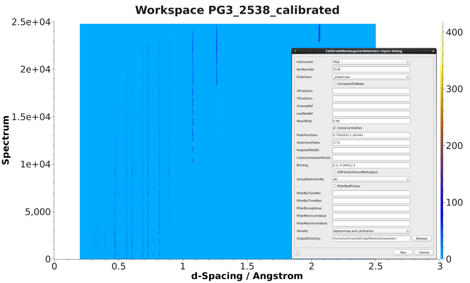
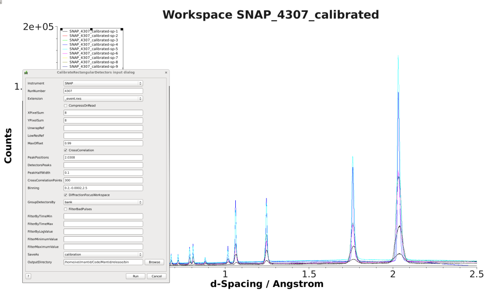
The OutputCalibrationTable is a TableWorkspace. See below for how to save, load, and use the workspace.

Workflow algorithms ¶

CalibrateRectangularDetectors will do most of the workflow for you, including applying the calibration to the data. While its name suggests it is only for a particular subset of detector types, it is not. It has many options for selecting between GetDetectorOffsets and GetDetOffsetsMultiPeaks.

Saving and Loading Calibration ¶

There are two basic formats for the calibration information. The legacy ascii format is described in CalFile. The newer HDF5 version is described alongside the description of calibration table.

Saving and loading the HDF5 format is done with SaveDiffCal and LoadDiffCal.

Saving and loading the legacy format is done with SaveCalFile and LoadCalFile. This can be converted from an OffsetsWorkspace to a calibration table using ConvertDiffCal.

Testing your Calibration ¶

The first thing that should be done is to convert the calibration workspace (either table or OffsetsWorkspace to a workspace of \(DIFC\) values to inspect using the instrument view. This can be done using CalculateDIFC. The values of \(DIFC\) should vary continuously across the detectors that are close to each other (e.g. neighboring pixels in an LPSD).

You will need to test that the calibration managed to find a reasonable calibration constant for each of the spectra in your data. The easiest way to do this is to apply the calibration to your calibration data and check that the bragg peaks align as expected.

Load the calibration data using Load
Run AlignDetectors, this will convert the data to d-spacing and apply the calibration. You can provide the calibration using the CalibrationFile, the CalibrationWorkspace, or OffsetsWorkspace.
Plot the workspace as a Color Fill plot, in the spectrum view, or a few spectra in a line plot.

Further insight can be gained by comparing the grouped (after aligning and focussing the data) spectra from a previous calibration or convert units to the newly calibrated version. This can be done using AlignAndFocusPowder with and without calibration information. In the end, a Rietveld refinement is the best test of the calibration.

Expanding on detector masking ¶

While many of the calibration methods will generate a mask based on the detectors calibrated, sometimes additional metrics for masking are desired. One way is to use DetectorDiagnostic. The result can be combined with an existing mask using

BinaryOperateMasks(InputWorkspace1='mask_from_cal', InputWorkspace2='mask_detdiag',
                   OperationType='OR', OutputWorkspace='mask_final')

Creating detector grouping ¶

To create a grouping workspace for SaveDiffCal you need to specify which detector pixels to combine to make an output spectrum. This is done using CreateGroupingWorkspace. An alternative is to generate a grouping file to load with LoadDetectorsGroupingFile.

Adjusting the Instrument Definition ¶

This approach attempts to correct the instrument component positions based on the calibration data. It can be more involved than applying the correction during focussing.

Perform a calibration using CalibrateRectangularDetectors or GetDetOffsetsMultiPeaks. Only these algorithms can export the Diffraction Calibration Workspace required.
Run AlignComponents this will move aspects of the instrument to optimize the offsets. It can move any named aspect of the instrument including the sample and source positions. You will likely need to run this several times, perhaps focussing on a single bank at a time, and then the source and sample positions in order to get a good alignment.
Then either:
- ExportGeometry will export the resulting geometry into a format that can be used to create a new XML instrument definition. The Mantid team at ORNL have tools to automate this for some instruments at the SNS.
- At ISIS enter the resulting workspace as the calibration workspace into the DAE software when recording new runs. The calibrated workspace will be copied into the resulting NeXuS file of the run.

Calibration Diagnostics ¶

Pixel-by-pixel results ¶

../../_images/VULCAN_192227_pixel_calibration.png

There are some common ways of diagnosing the calibration results. One of the more common is to plot the aligned data in d-spacing. While this can be done via the “colorfill” plot or sliceviewer, a function has been created to annotate the plot with additional information. This can be done using the following code

from mantid.simpleapi import (AlignDetectors, LoadDiffCal, LoadEventNexus, LoadInstrument, Rebin)
from Calibration.tofpd import diagnostics

LoadEventNexus(Filename='VULCAN_192227.nxs.h5', OutputWorkspace='ws')
Rebin(InputWorkspace='ws', OutputWorkspace='ws', Params=(5000,-.002,70000))
LoadDiffCal(Filename='VULCAN_Calibration_CC_4runs_hybrid.h5', InputWorkspace='ws', WorkspaceName='VULCAN')
AlignDetectors(InputWorkspace='ws', OutputWorkspace='ws', CalibrationWorkspace='VULCAN_cal')
diagnostics.plot2d(mtd['ws'], horiz_markers=[8*512*20, 2*8*512*20], xmax=1.3)

Here the expected peak positions are vertical lines, the horizontal lines are boundaries between banks. When run interactively, the zoom/pan tools are available.

DIFC of unwrapped instrument ¶

To check the consistency of pixel-level calibration, the DIFC value of each pixel can be compared between two different instrument calibrations. The percent change in DIFC value is plotted over a view of the unwrapped instrument where the horizontal and vertical axis corresponds to the polar and azimuthal angle, respectively. The azimuthal angle of 0 corresponds to the direction parallel of the positive Y-axis in 3D space.

Below is an example of the change in DIFC between two different calibrations of the NOMAD instrument.

../../_images/NOMAD_difc_calibration.png

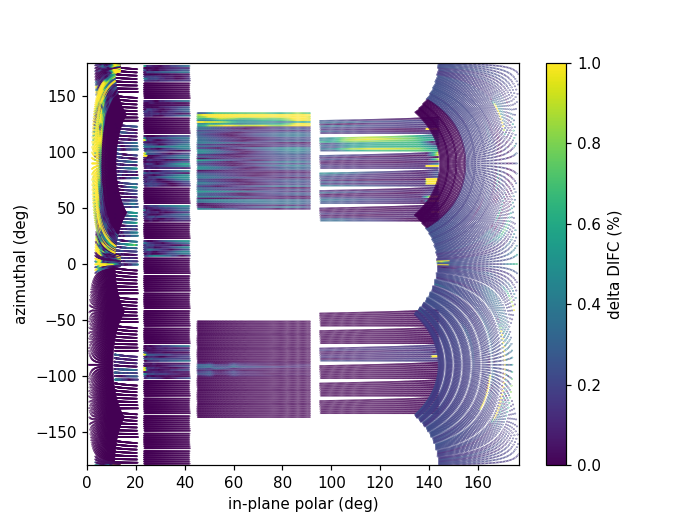
This plot can be generated several different ways: by using calibration files, calibration workspaces, or resulting workspaces from CalculateDIFC. The first input parameter is always required and represents the new calibration. The second parameter is optional and represents the old calibration. When it is not specified, the default instrument geometry is used for comparison. Masks can be included by providing a mask using the mask parameter. To control the scale of the plot, a tuple of the minimum and maximum percentage can be specified for the vrange parameter.

from Calibration.tofpd import diagnostics

# Use filenames to generate the plot
fig, ax = diagnostics.difc_plot2d("NOM_calibrate_d135279_2019_11_28.h5", "NOM_calibrate_d131573_2019_08_18.h5")

When calibration tables are used as inputs, an additional workspace parameter is needed (instr_ws) to hold the instrument definition. This can be the GroupingWorkspace generated with the calibration tables from LoadDiffCal as seen below.

from mantid.simpleapi import LoadDiffCal
from Calibration.tofpd import diagnostics

# Use calibration tables to generate the plot
LoadDiffCal(Filename="NOM_calibrate_d135279_2019_11_28.h5", WorkspaceName="new")
LoadDiffCal(Filename="NOM_calibrate_d131573_2019_08_18.h5", WorkspaceName="old")
fig, ax = diagnostics.difc_plot2d("new_cal", "old_cal", instr_ws="new_group")

Finally, workspaces with DIFC values can be used directly:

from mantid.simpleapi import CalculateDIFC, LoadDiffCal
from Calibration.tofpd import diagnostics

# Use the results from CalculateDIFC directly
LoadDiffCal(Filename="NOM_calibrate_d135279_2019_11_28.h5", WorkspaceName="new")
LoadDiffCal(Filename="NOM_calibrate_d131573_2019_08_18.h5", WorkspaceName="old")
difc_new = CalculateDIFC(InputWorkspace="new_group", CalibrationWorkspace="new_cal")
difc_old = CalculateDIFC(InputWorkspace="old_group", CalibrationWorkspace="old_cal")
fig, ax = diagnostics.difc_plot2d(difc_new, difc_old)

A mask can also be applied with a MaskWorkspace to hide pixels from the plot:

from mantid.simpleapi import LoadDiffCal
from Calibration.tofpd import diagnostics

# Use calibration tables to generate the plot
LoadDiffCal(Filename="NOM_calibrate_d135279_2019_11_28.h5", WorkspaceName="new")
LoadDiffCal(Filename="NOM_calibrate_d131573_2019_08_18.h5", WorkspaceName="old")
fig, ax = diagnostics.difc_plot2d("new_cal", "old_cal", instr_ws="new_group", mask="new_mask")

Relative Strain ¶

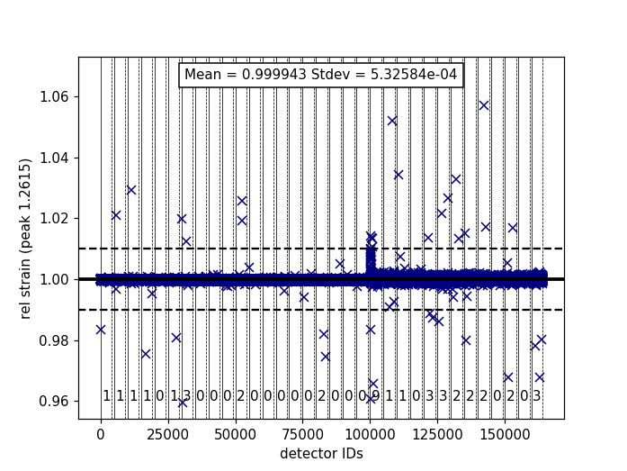
Plotting the relative strain of the d-spacing for a peak to the nominal d value (\(\frac{observed}{expected}\)) can be used as another method to check the calibration consistency at the pixel level. The relative strain is plotted along the Y-axis for each detector pixel, with the mean and standard deviation reported on the plot. A solid black line is drawn at the mean, and two dashed lines are drawn above and below the mean by a threshold percentage (one percent of the mean by default). This can be used to determine which pixels are bad up to a specific threshold.

Below is an example of the relative strain plot for VULCAN at peak position 1.2615:

../../_images/VULCAN_relstrain_diagnostic.png

The plot shown above can be generated from the following script:

import numpy as np
from mantid.simpleapi import (LoadEventAndCompress, LoadInstrument, PDCalibration, Rebin)
from Calibration.tofpd import diagnostics

FILENAME = 'VULCAN_192227.nxs.h5'
CALFILE = 'VULCAN_Calibration_CC_4runs_hybrid.h5'

peakpositions = np.asarray(
  (0.3117, 0.3257, 0.3499, 0.3916, 0.4205, 0.4645, 0.4768, 0.4996, 0.515, 0.5441, 0.5642, 0.6307, 0.6867,
   0.7283, 0.8186, 0.892, 1.0758, 1.2615, 2.06))

LoadEventAndCompress(Filename=FILENAME, OutputWorkspace='ws', FilterBadPulses=0)
LoadInstrument(Workspace='ws', InstrumentName="VULCAN", RewriteSpectraMap='True')
Rebin(InputWorkspace='ws', OutputWorkspace='ws', Params=(5000, -.002, 70000))

PDCalibration(InputWorkspace='ws', TofBinning=(5000,-.002,70000),
              PeakPositions=peakpositions,
              MinimumPeakHeight=5,
              OutputCalibrationTable='calib',
              DiagnosticWorkspaces='diag')

dspacing = diagnostics.collect_peaks('diag_dspacing', 'dspacing', donor='diag_fitted',
                                     infotype='dspacing')
strain = diagnostics.collect_peaks('diag_dspacing', 'strain', donor='diag_fitted')

fig, ax = diagnostics.plot_peakd('strain', 1.2615, drange=(0, 200000), plot_regions=True, show_bad_cnt=True)

To plot the relative strain for multiple peaks, an array of positions can be passed instead of a single value. For example, using peakpositions in place of 1.2615 in the above example results in the relative strain for all peaks being plotted as shown below.

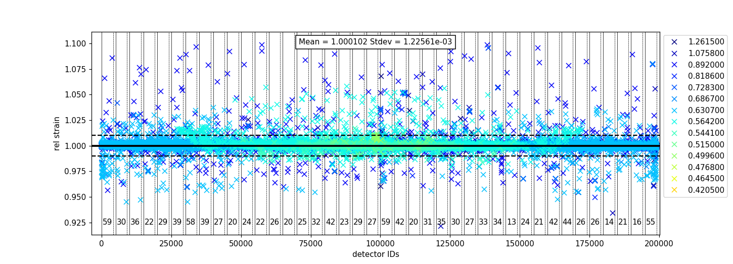
The vertical lines shown in the plot are drawn between detector regions and can be used to report the count of bad pixels found in each region. The solid vertical line indicates the start of a region, while the dashed vertical line indicates the end of a region. The vertical lines can be turned off with plot_regions=False and displaying the number of bad counts for each region can also be disabled with show_bad_cnt=False. When plot_regions=False but show_bad_cnt=True, a single count of bad pixels over the entire range is shown at the bottom center of the plot.

As seen in the above example, the x-range of the plot can be narrowed down using the drange option, which accepts a tuple of the starting detector ID and ending detector ID to plot.

To adjust the horizontal bars above and below the mean, a percent can be passed to the threshold option.

Pearson Correlation Coefficient ¶

It can be useful to compare the linearity of the relationship between time of flight and d-spacing for each peak involved in calibration. In theory, the relationship between (TOF, d-spacing) will always be perfectly linear, but in practice, that is not always the case. This diagnostic plot primarily serves as a tool to ensure that the calibration makes sense, i.e., that a single DIFC parameter is enough to do the transformation. In the ideal case, all Pearson correlation coefficients will be close to 1. For more on Pearson correlation coefficients please see this wikipedia article. Below is an example plot for the Pearson correlation coefficient of (TOF, d-spacing).

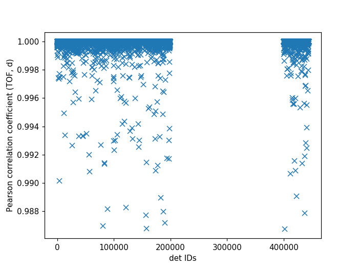
The following script can be used to generate the above plot.

# import mantid algorithms, numpy and matplotlib
from mantid.simpleapi import *
import matplotlib.pyplot as plt
import numpy as npfrom Calibration.tofpd import diagnosticsFILENAME = 'VULCAN_192226.nxs.h5'  # 88 sec

FILENAME = 'VULCAN_192227.nxs.h5'  # 2.8 hour
CALFILE = 'VULCAN_Calibration_CC_4runs_hybrid.h5'peakpositions = np.asarray(
  (0.3117, 0.3257, 0.3499, 0.3916, 0.4205, 0.4645, 0.4768, 0.4996, 0.515, 0.5441, 0.5642, 0.6307, 0.6867,
   0.7283, 0.8186, 0.892, 1.0758, 1.2615, 2.06))

peakpositions = peakpositions[peakpositions > 0.4]
peakpositions = peakpositions[peakpositions < 1.5]
peakpositions.sort()LoadEventAndCompress(Filename=FILENAME, OutputWorkspace='ws', FilterBadPulses=0)

LoadInstrument(Workspace='ws', Filename="mantid/instrument/VULCAN_Definition.xml", RewriteSpectraMap='True')
Rebin(InputWorkspace='ws', OutputWorkspace='ws', Params=(5000, -.002, 70000))
PDCalibration(InputWorkspace='ws', TofBinning=(5000,-.002,70000),
           PeakPositions=peakpositions,
           MinimumPeakHeight=5,
           OutputCalibrationTable='calib',
           DiagnosticWorkspaces='diag')
center_tof = diagnostics.collect_fit_result('diag_fitparam', 'center_tof', peakpositions, donor='ws', infotype='centre')
fig, ax = diagnostics.plot_corr('center_tof')

Peak Information ¶

Plotting the fitted peak parameters for different instrument banks can also provide useful information for calibration diagnostics. The fitted peak parameters from FitPeaks (center, width, height, and intensity) are plotted for each bank at different peak positions. This can be used to help calibrate each group rather than individual detector pixels.

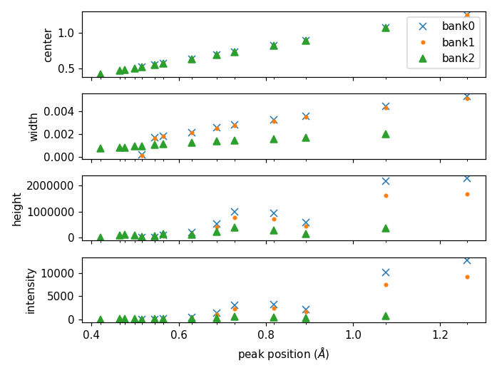
../../_images/VULCAN_peakinfo_diagnostic.png

The above figure can be generated using the following script:

import numpy as np
from mantid.simpleapi import (AlignAndFocusPowder, ConvertUnits, FitPeaks, LoadEventAndCompress,
                              LoadDiffCal, LoadInstrument)
from Calibration.tofpd import diagnostics

FILENAME = 'VULCAN_192227.nxs.h5'  # 2.8 hour
CALFILE = 'VULCAN_Calibration_CC_4runs_hybrid.h5'

peakpositions = np.asarray(
    (0.3117, 0.3257, 0.3499, 0.3916, 0.4205, 0.4645, 0.4768, 0.4996, 0.515, 0.5441, 0.5642, 0.6307, 0.6867,
     0.7283, 0.8186, 0.892, 1.0758, 1.2615, 2.06))
peakpositions = peakpositions[peakpositions > 0.4]
peakpositions = peakpositions[peakpositions < 1.5]
peakpositions.sort()
peakwindows = diagnostics.get_peakwindows(peakpositions)

LoadEventAndCompress(Filename=FILENAME, OutputWorkspace='ws', FilterBadPulses=0)
LoadInstrument(Workspace='ws', InstrumentName="VULCAN", RewriteSpectraMap='True')

LoadDiffCal(Filename=CALFILE, InputWorkspace='ws', WorkspaceName='VULCAN')
AlignAndFocusPowder(InputWorkspace='ws',
                    OutputWorkspace='focus',
                    GroupingWorkspace="VULCAN_group",
                    CalibrationWorkspace="VULCAN_cal",
                    MaskWorkspace="VULCAN_mask",
                    Dspacing=True,
                    Params="0.3,3e-4,1.5")

ConvertUnits(InputWorkspace='focus', OutputWorkspace='focus', Target='dSpacing', EMode='Elastic')
FitPeaks(InputWorkspace='focus',
        OutputWorkspace='output',
        PeakFunction='Gaussian',
        RawPeakParameters=False,
        HighBackground=False,  # observe background
        ConstrainPeakPositions=False,
        MinimumPeakHeight=3,
        PeakCenters=peakpositions,
        FitWindowBoundaryList=peakwindows,
        FittedPeaksWorkspace='fitted',
        OutputPeakParametersWorkspace='parameters')

fig, ax = diagnostics.plot_peak_info('parameters', peakpositions)

Category: Calibration