\(\renewcommand\AA{\unicode{x212B}}\)
Exercises
Exercise 1
- Load the EventWorkspace HYS_11388_event.nxs
- Sum across each spectra in the workspace using the SumSpectra
algorithm. Set the OutputWorkspace to be called Sum
- Rebin this grouped workspace, specify OutputWorkspace to
binned and that the bin width is 100 microseconds, and keep
PreserveEvents ticked
- Right-click the workspace called binned and choose the Plot
Spectrum option. Once the graph is plotted, leave do not delete it
- Events in an EventWorkspace may get filtered according to other
recorded events during the experiments. At perhaps the simplest level
you can filter out events between specific times. Use
FilterByTime v1 for this. It has a parameter called
StartTime, which is the start time, in seconds, since the start
of the run. Events before this time are filtered out. Run
FilterByTime on binned with StartTime=4000 and call the
OutputWorkspace FilteredByTime
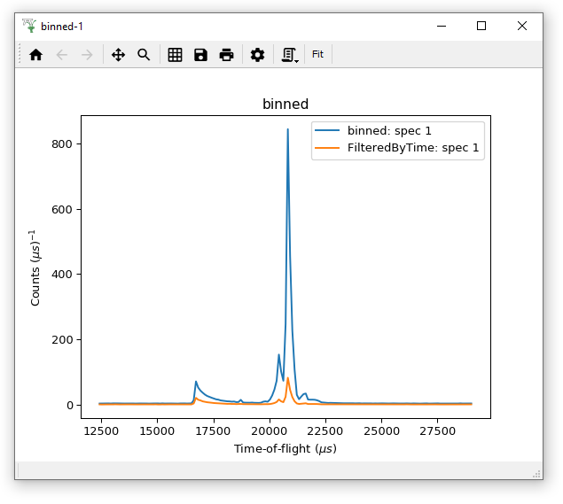
- Drag the workspace FilteredByTime into the plot where workspace
binned is plotted. What you should see now is:
Show the History of the FilteredByTime workspace, which should match the steps above.
Exercise 2
- Using the binned workspace from the previous example as the
InputWorkspace, use FilterByLogValue with
LogName=proton_charge, MinimumValue=17600000,
MaximumValue=17890000
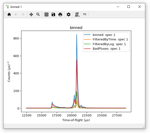
- Overplot the OutputWorkspace over your existing plots from the
previous example
- Run FilterBadPulses with InputWorkspace=binned and
LowerCutoff=99.999
- Overplot the OutputWorkspace over your existing plots
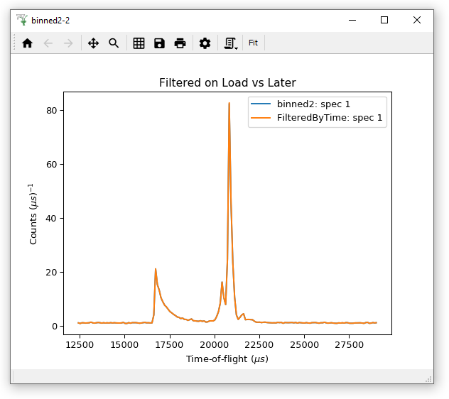
Exercise 3 - now you choose the OutputWorkspace names!
- Load HYS_11388_event.nxs as in Exercise 1, but this time perform
the filtering as part of the Loading, by setting FilterByTimeStart=4000
- SumSpectra on your new workspace
- Use RebinToWorkspace to achieve the same binning as the existing
binned workspace
- Plot both your newly rebinned workspace and FilteredByTime created
in exercise 1 on a new plot.