\(\renewcommand\AA{\unicode{x212B}}\)
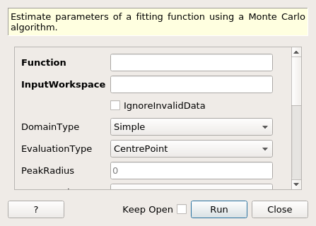
EstimateFitParameters dialog.
Table of Contents
| Name | Direction | Type | Default | Description |
|---|---|---|---|---|
| Function | InOut | Function | Mandatory | Parameters defining the fitting function and its initial values |
| InputWorkspace | Input | Workspace | Mandatory | Name of the input Workspace |
| IgnoreInvalidData | Input | boolean | False | Flag to ignore infinities, NaNs and data with zero errors. |
| DomainType | Input | string | Simple | The type of function domain to use: Simple, Sequential, or Parallel. Allowed values: [‘Simple’, ‘Sequential’, ‘Parallel’] |
| EvaluationType | Input | string | CentrePoint | The way the function is evaluated on histogram data sets. If value is “CentrePoint” then function is evaluated at centre of each bin. If it is “Histogram” then function is integrated within the bin and the integrals returned. Allowed values: [‘CentrePoint’, ‘Histogram’] |
| PeakRadius | Input | number | 0 | A value of the peak radius the peak functions should use. A peak radius defines an interval on the x axis around the centre of the peak where its values are calculated. Values outside the interval are not calculated and assumed zeros.Numerically the radius is a whole number of peak widths (FWHM) that fit into the interval on each side from the centre. The default value of 0 means the whole x axis. |
| CostFunction | InOut | string | Least squares | The cost function to be used for the fit, default is Least squares. Allowed values: [‘Least squares’, ‘Poisson’, ‘Rwp’, ‘Unweighted least squares’] |
| NSamples | Input | number | 100 | Number of samples. |
| Constraints | Input | string | Additional constraints on tied parameters. | |
| Type | Input | string | Monte Carlo | Type of the algorithm: “Monte Carlo” or “Cross Entropy” |
| NOutputs | Input | number | 10 | Number of parameter sets to output to OutputWorkspace. Unused if OutputWorkspace isn’t set. (Monte Carlo only) |
| OutputWorkspace | Output | TableWorkspace | Optional: A table workspace with parameter sets producing the smallest values of cost function. (Monte Carlo only) | |
| NIterations | Input | number | 10 | Number of iterations of the Cross Entropy algorithm. |
| Selection | Input | number | 10 | Size of the selection in the Cross Entropy algorithm from which to estimate new distribution parameters for the next iteration. |
| FixBadParameters | Input | boolean | False | If true try to estimate which parameters may cause problems for fitting and fix them. |
| Seed | Input | number | 0 | A seed value for the random number generator. The default value (0) makes the generator use a random seed. |
This algorithm uses a Monte Carlo - type approach to estimate initial values of function parameters before passing the function to Fit v1 algorithm. The user needs to provide the search intervals for each parameters that requires estimation. These intervals are set by defining boundary constraints in the fitting function. For example:
name=UserFunction,Formula=a*x+b,a=0,b=0,constraints=(1<a<4, 0<b<4)
Here the algorithm will search intervals [1, 4] and [0, 4] for values of parameters a and b respectively such that the cost function is the smallest.
If a parameter will be fixed or tied in a fit don’t include it in the constraints. For example:
name=UserFunction,Formula=a*x+b,a=0,ties=(b=1.9),constraints=(1<a<4)
name=UserFunction,Formula=a*x+b,a=0,ties=(b=a-1),constraints=(1<a<4)
The algorithm uses one of the two strategies (set via Type property): “Monte Carlo” and “Cross Entropy”.
In this strategy a number (defined by NSamples property) of parameter sets are generated and the one that gives the smallest cost function is considered the winner. These best parameters are set to Function property (it has the InOut direction).
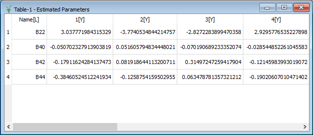
If OutputWorkspace property is set then more than 1 parameter set can be output. The output workspace is a table workspace in which the first column contains the names of the parameters and the subsequent columns have the parameter sets with the smallest cost fnction values. Below is an example of such a workspace.
This strategy iteratively tries to narrow down the search space using statistics from a previous iteration.
The steps of the algorithm:
It may happen that some of the parameters cannot be determined from the data set in the InputWorkspace. If this is the case Fit v1 may diverge or fail with an error. To try and find such parameters set FixBadParameters to true. If the algorithm decides that some of the parameters may cause problems it will fix them.
Example 1.
# Create a data set. It is a BackToBackExponential.
x = [-8.4, -7.4, -6.4, -5.4, -4.4, -3.4, -2.4, -1.4, -0.4, 0.6, 1.6, 2.6, 3.6, 4.6, 5.6, 6.6, 7.6, 8.5]
y = [5.899424685451e-06, 0.0007065291085075, 0.03312893859911,
0.6260554060356, 4.961949842664, 17.4766663495,
30.00494980772, 29.34773951093, 20.53693564978,
12.73990150587, 7.739398423952, 4.694362241084,
2.847186128946, 1.726807862958, 1.047276595461,
0.6351380161499, 0.3851804649058, 0.1957211887562]
ws = CreateWorkspace(x, y)
# Define a function, constraints set the search intervals.
fun = 'name=BackToBackExponential,S=1.1,constraints=(50<I<200,0.1<A<300,0.01<B<10,-5<X0<0,0.001<S<4)'
# Set up the algorithm.
from mantid.api import AlgorithmManager
alg = AlgorithmManager.createUnmanaged('EstimateFitParameters')
alg.initialize()
alg.setProperty('Function', fun)
alg.setProperty('InputWorkspace', ws)
# Non-default cost function can be used.
alg.setProperty('CostFunction', 'Unweighted least squares')
# How many points to try.
alg.setProperty('NSamples', 1000)
# A seed for the random number generator. Only to make this test reproducible.
alg.setProperty('Seed', 1234)
# Execute the algorithm.
alg.execute()
# Function now contains the estimated parameters.
function = alg.getProperty('Function').value
print(function)
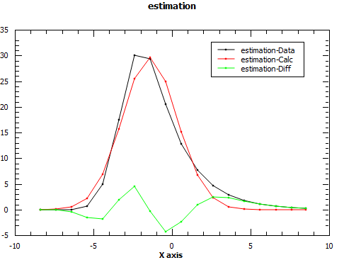
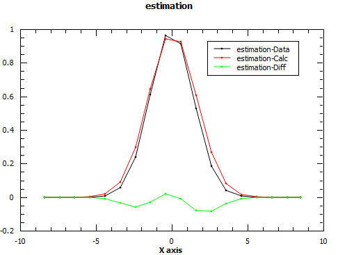
# Evaluate the function with the returned parameters to see the quality of estimation.
EvaluateFunction(str(function),ws,OutputWorkspace='estimation')
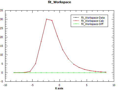
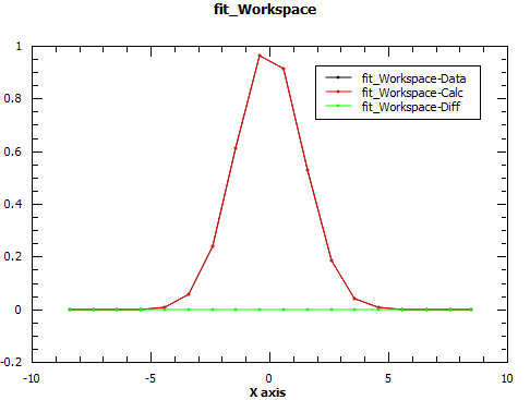
# Run Fit starting with the new parameters.
Fit(str(function),ws,Output='fit')
Output:
(You may see different numbers for the parameters when you run this example on your machine.)
name=BackToBackExponential,I=...,A=...,B=...,X0=...,S=...,constraints=(50<I<200,0.1<A<300,0.01<B<10,-5<X0<0,0.001<S<4)
Example 2.
# Create a data set. It is a Gaussian.
x = [-8.4, -7.4, -6.4, -5.4, -4.4, -3.4, -2.4, -1.4, -0.4, 0.6,  1.6,  2.6,  3.6,  4.6,  5.6,  6.6,  7.6,  8.5]
y = [2.18295779512548e-08, 1.13372713874796e-06, 3.57128496416351e-05,
    0.000682328052756376, 0.00790705405159343, 0.0555762126114831,
    0.236927758682122, 0.612626394184416, 0.960789439152323,
    0.913931185271228, 0.527292424043049, 0.184519523992989,
    0.0391638950989871, 0.00504176025969098, 0.000393669040655079,
    1.86437423315169e-05, 5.35534780279311e-07, 1.43072419185677e-08]
ws = CreateWorkspace(x, y)

# Define a function, constraints set the search intervals.
fun = 'name=BackToBackExponential,S=1.1,constraints=(0.01<I<200,0.001<A<300,0.001<B<300,-5<X0<5,0.001<S<4)'

# Set up the algorithm.
from mantid.api import AlgorithmManager
alg = AlgorithmManager.createUnmanaged('EstimateFitParameters')
alg.initialize()
alg.setProperty('Function', fun)
alg.setProperty('InputWorkspace', ws)
# Cross Entropy type.
alg.setProperty('Type', 'Cross Entropy')
# How many samples in each iteration.
alg.setProperty('NSamples', 100)
# How many samples to use to refine distributions.
alg.setProperty('Selection', 10)
# How many iterations to make.
alg.setProperty('NIterations', 10)
# Try to find bad parameters. A and B are expected to be bad.
alg.setProperty('FixBadParameters', True)
# A seed for the random number generator. Only to make this test reproducible.
alg.setProperty('Seed', 1234)
# Execute the algorithm.
alg.execute()
# Function now contains the estimated parameters.
function = alg.getProperty('Function').value
print(function)
# Evaluate the function with the returned parameters to see the quality of estimation.
EvaluateFunction(str(function),ws,OutputWorkspace='estimation')
# Run Fit starting with the new parameters.
Fit(str(function),ws,Output='fit')
Output:
(You may see different numbers for the parameters when you run this example on your machine.)
name=BackToBackExponential,I=...,X0=...,S=...,constraints=(0.01<I<200,0.001<A<300,0.001<B<300,-5<X0<5,0.001<S<4),ties=(A=...,B=...)
Categories: AlgorithmIndex | Optimization