\(\renewcommand\AA{\unicode{x212B}}\)
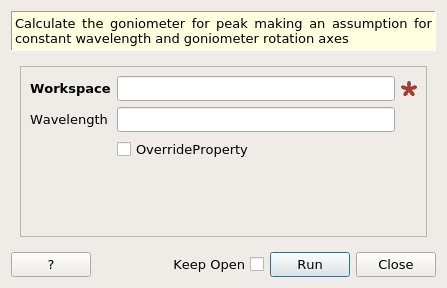
HFIRCalculateGoniometer dialog.
Table of Contents
Calculate the goniometer for peak making an assumption for constant wavelength and goniometer rotation axes
| Name | Direction | Type | Default | Description |
|---|---|---|---|---|
| Workspace | InOut | IPeaksWorkspace | Mandatory | Peaks Workspace to be modified |
| Wavelength | Input | number | Optional | Wavelength to set the workspace, will be the value set on workspace if not provided. |
| OverrideProperty | Input | boolean | False | If False then the value for InnerGoniometer and FlipX will be determiend from the workspace, it True then the properties will be used |
| InnerGoniometer | Input | boolean | False | Whether the goniometer to be calculated is the most inner (phi) or most outer (omega) |
| FlipX | Input | boolean | False | Used when calculating goniometer angle if the q_lab x value should be negative, hence the detector of the other side (right) of the beam |
This algorithm calculates the goniometer of peaks from the q_sample
and wavelength. It makes use of the
mantid.geometry.Goniometer.calcFromQSampleAndWavelength()
method. It was created to work with WAND² (HB2C) and DEMAND (HB3A) at
HFIR but may be applied to other constant wavelength instruments.
The wavelength will be read from the workspace property wavelength unless one is provided as input. The peaks with have their wavelength set to this value.
The goniometer is calculated by the following method. It only works for a constant wavelength source. It also assumes the goniometer rotation is around the y-axis only.
You can specify if the goniometer to calculated is omega or phi, outer or inner respectively, by setting the option InnerGoniometer. The existing goniometer on the workspace will be used as the starting goniometer allowing only the scanning goniometer to be calculated. This won’t change anything for HB2C as they only have an omega axis but for HB3A you need to make sure that the goniometer is correctly set from the logs with SetGoniometer(Workspace=scan, Axis0=’omega,0,1,0,-1’, Axis1=’chi,0,0,1,-1’, Axis2=’phi,0,1,0,-1’) and that you can only process peak workspaces containing peaks from a single scan at a time.
The goniometer (\(G\)) is calculated from \(\textbf{Q}_{sample}\) for a given wavelength (\(\lambda\)) by:
First calculate the \(\textbf{Q}_{lab}\) using \(\textbf{Q}_{sample}\) and \(\lambda\).
\(\therefore\)
where \(\theta\) is from 0 to \(\pi\) and \(\phi\) is from \(-\pi/2\) to \(\pi/2\). This means that it will assume your detector position is on the left of the beam even if it’s not, unless the option FlipX is set to True then the \(\textbf{Q}_{lab}^x = -\textbf{Q}_{lab}^x\).
Now you have \(\theta\), \(\phi\) and k you can get \(\textbf{Q}_{lab}\) using (1).
We need to now solve \(G \textbf{Q}_{sample} = \textbf{Q}_{lab}\). For a rotation around y-axis only we want to find \(\psi\) for:
which gives two equations
make
Then we need to solve \(A X = B\) for \(X\) where
then
Put \(\psi\) into (2) and you have the goniometer for that peak.
Note
If the instrument is HB3A and the InnerGoniometer and FlipX properties are left empty then these values will be set correctly automatically.
Example: omega calculation
peaks = CreatePeaksWorkspace(OutputType="LeanElasticPeak", NumberOfPeaks=0)
peaks.addPeak(peaks.createPeakQSample([0.5, 0, np.sqrt(3)/2]))   # omega = -90
peaks.addPeak(peaks.createPeakQSample([0, 0, 1]))                # omega = -60
peaks.addPeak(peaks.createPeakQSample([-0.5, 0, np.sqrt(3)/2]))  # omega = -30
peaks.addPeak(peaks.createPeakQSample([-np.sqrt(3)/2, 0, 0.5]))  # omega = 0
peaks.addPeak(peaks.createPeakQSample([-1, 0, 0]))               # omega = 30
peaks.addPeak(peaks.createPeakQSample([-np.sqrt(3)/2, 0, -0.5])) # omega = 60
peaks.addPeak(peaks.createPeakQSample([-0.5, 0, -np.sqrt(3)/2])) # omega = 90
HFIRCalculateGoniometer(peaks, 2*np.pi)
for n in range(7):
    g = Goniometer()
    g.setR(peaks.getPeak(n).getGoniometerMatrix())
    print(f"Peak {n} - omega = {g.getEulerAngles('YZY')[0]:.1f}")
Output:
Peak 0 - omega = -90.0
Peak 1 - omega = -60.0
Peak 2 - omega = -30.0
Peak 3 - omega = 0.0
Peak 4 - omega = 30.0
Peak 5 - omega = 60.0
Peak 6 - omega = 90.0
Categories: AlgorithmIndex | Diffraction\Reduction
Python: HFIRCalculateGoniometer.py