\(\renewcommand\AA{\unicode{x212B}}\)

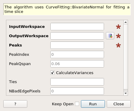
IntegratePeakTimeSlices v1¶

IntegratePeakTimeSlices dialog.

Table of Contents

Summary
- See Also
Properties
Description
Usage
Source

Summary ¶

The algorithm uses CurveFitting::BivariateNormal for fitting a time slice

Properties ¶

Name	Direction	Type	Default	Description
InputWorkspace	Input	MatrixWorkspace	Mandatory	A 2D workspace with X values of time of flight
OutputWorkspace	Output	TableWorkspace		Name of the output table workspace with Log info
Peaks	Input	PeaksWorkspace	Mandatory	Workspace of Peaks
PeakIndex	Input	number	0	Index of peak in PeaksWorkspace to integrate
PeakQspan	Input	number	0.06	Max magnitude of Q of Peak to Q of Peak Center, where mod(Q)=1/d
CalculateVariances	Input	boolean	True	Calc (co)variances given parameter values versus fit (co)Variances
Ties	Input	string		Tie parameters(Background,Intensity, Mrow,…) to values/formulas.
NBadEdgePixels	Input	number	0	Number of bad Edge Pixels
Intensity	Output	number		Peak Integrated Intensity
SigmaIntensity	Output	number		Peak Integrated Intensity Error

Description ¶

This algorithm fits a bivariate normal distribution( plus background) to the data on each time slice. The Fit program uses BivariateNormal for the Fit Function.

The area used for the fitting is calculated based on the dQ parameter. A good value for dQ is 1/largest unit cell length. This parameter dictates the size of the area used to approximate the intensity of the peak. The estimate .1667/ max(a,b,c) assumes |Q|=1/d.

The result is returned in this algorithm’s output “Intensity” and “SigmaIntensity” properties. The peak object is NOT CHANGED.

The table workspace is also a result. Each line contains information on the fit for each good time slice. The column names( and information) in the table are:

`` Time, Channel, Background, Intensity, Mcol, Mrow, SScol,SSrow, SSrc, NCells,``
`` ChiSqrOverDOF, TotIntensity, BackgroundError, FitIntensityError, ISAWIntensity,``
``  ISAWIntensityError,TotalBoundary, NBoundaryCells, Start Row, End Row,Start Col, and End Col.``
``  The last column has a comma separated List of sepctral ID’s used in the time slice.``

The final Peak intensity is the sum of the IsawIntensity for each time slice. The error is the square root of the sum of squares of the IsawIntensityError values.

The columns whose names are Background, Intensity, Mcol, Mrow, SScol, SSrow, and SSrc correspond to the parameters for the BivariateNormal curve fitting function.

This algorithm has been carefully tweaked to give good results for interior peaks only. Peaks close to the edge of the detector may not give good results.

This Algorithm is also used by the PeakIntegration v1 algorithm when the Fit tag is selected.

Usage ¶

# Load a SCD data set from systemtests Data and find the peaks
LoadEventNexus(Filename=r'TOPAZ_3132_event.nxs',OutputWorkspace='TOPAZ_3132_nxs')
ConvertToDiffractionMDWorkspace(InputWorkspace='TOPAZ_3132_nxs',OutputWorkspace='TOPAZ_3132_md',LorentzCorrection='1')
FindPeaksMD(InputWorkspace='TOPAZ_3132_md',PeakDistanceThreshold='0.15',MaxPeaks='100',OutputWorkspace='peaks')
FindUBUsingFFT(PeaksWorkspace='peaks',MinD='2',MaxD='16')
IndexPeaks(PeaksWorkspace='peaks')

# Run the Integration algorithm and print results
peak0,int,sig = IntegratePeakTimeSlices(InputWorkspace='TOPAZ_3132_nxs', Peaks='peaks', Intensity=4580.8587719746683, SigmaIntensity=190.21154129339735)
print("Intensity and SigmaIntensity of peak 0  = {} {}".format(int, sig))