\(\renewcommand\AA{\unicode{x212B}}\)
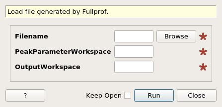
LoadFullprofFile dialog.
Table of Contents
| Name | Direction | Type | Default | Description |
|---|---|---|---|---|
| Filename | Input | string | Mandatory | Name of [http://www.ill.eu/sites/fullprof/ Fullprof] .hkl or .prf file. Allowed extensions: [‘.hkl’, ‘.prf’, ‘.dat’] |
| PeakParameterWorkspace | Output | TableWorkspace | Mandatory | Name of table workspace containing peak parameters from .hkl file. |
| OutputWorkspace | Output | MatrixWorkspace | Mandatory | Name of data workspace containing the diffraction pattern in .prf file. |
This algorithm is to import Fullprof .irf file (peak parameters) and .hkl file (reflections) and record the information to TableWorkspaces, which serve as the inputs for algorithm LeBailFit.
Instrument parameter TableWorkspace contains all the peak profile parameters imported from Fullprof .irf file.
Presently these are the peak profiles supported
* Thermal neutron back to back exponential convoluted with pseudo-voigt (profile No. 10 in Fullprof)
Each row in TableWorkspace corresponds to one profile parameter.
Columns include Name, Value, FitOrTie, Min, Max and StepSize.
Each row of this workspace corresponds to one diffraction peak. The information contains the peak’s Miller index and (local) peak profile parameters of this peak. For instance of a back-to-back exponential convoluted with Gaussian peak, the peak profile parameters include Alpha, Beta, Sigma, centre and height.
This algorithm is designed to work with other algorithms to do Le Bail fit. The introduction can be found in the wiki page of LeBailFit v1.
Example - load a Fullprof .prf file:
LoadFullprofFile(Filename=r'LaB6_1bank3_C.prf',
    PeakParameterWorkspace='LaB6_InfoTable',
    OutputWorkspace='PG3_LaB6_Bank3')

infotablews = mtd["LaB6_InfoTable"]
dataws = mtd["PG3_LaB6_Bank3"]

print("LaB6: A = B = C = {:.5f}, Alpha = Beta = Gamma = {:.5f}".format(infotablews.column('Value')[infotablews.column('Name').index('A')],
                                                                       infotablews.column('Value')[infotablews.column('Name').index('Alpha')]))

maxy = max(dataws.readY(1))
print("Maximum peak value (calculated) = {:.5f}".format(maxy))
Output:
Data set counter =  5431
Data Size =  5431
LaB6: A = B = C = 4.15689, Alpha = Beta = Gamma = 90.00000
Maximum peak value (calculated) = 13.38550
Example - load a Fullprof .irf file:
LoadFullprofFile(Filename=r'LB4854b3.hkl',
    PeakParameterWorkspace='LaB6_Ref_Table',
    OutputWorkspace='Fake')

fakedataws = mtd["Fake"]
reftablews = mtd["LaB6_Ref_Table"]

print("Reflection table imported {} peaks.  Faked data workspace contains {} data points.".format(
    reftablews.rowCount(), len(fakedataws.readX(0))))

index = 0
print("Peak {} of ({}, {}, {}): Alpha = {:.5f}, Beta = {:.5f}, FWHM = {:.5f}".format(index, reftablews.cell(index, 0),
    reftablews.cell(index, 1), reftablews.cell(index, 2), reftablews.cell(index, 3), reftablews.cell(index, 4), reftablews.cell(index, 7)))
index = 75
print("Peak {} of ({}, {}, {}): Alpha = {:.5f}, Beta = {:.5f}, FWHM = {:.5f}".format(index, reftablews.cell(index, 0),
    reftablews.cell(index, 1), reftablews.cell(index, 2), reftablews.cell(index, 3), reftablews.cell(index, 4), reftablews.cell(index, 7)))
Output:
Reflection table imported 76 peaks.  Faked data workspace contains 1 data points.
Peak 0 of (1, 1, 0): Alpha = 0.01963, Beta = 0.01545, FWHM = 289.07450
Peak 75 of (9, 3, 0): Alpha = 0.25569, Beta = 0.13821, FWHM = 14.67480
Categories: AlgorithmIndex | Diffraction\DataHandling
Python: LoadFullprofFile.py