\(\renewcommand\AA{\unicode{x212B}}\)
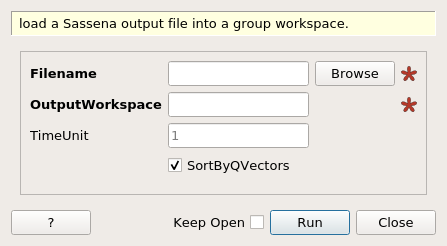
LoadSassena dialog.
Table of Contents
| Name | Direction | Type | Default | Description |
|---|---|---|---|---|
| Filename | Input | string | Mandatory | A Sassena file. Allowed extensions: [‘.h5’, ‘.hd5’] |
| OutputWorkspace | Output | Workspace | Mandatory | The name of the group workspace to be created. |
| TimeUnit | Input | number | 1 | The Time unit in between data points, in picoseconds. Default is 1.0 picosec. |
| SortByQVectors | Input | boolean | True | Sort structure factors by increasing momentum transfer? |
The Sassena application 1 generates intermediate scattering factors from molecular dynamics trajectories. This algorithm reads Sassena output and stores all data in workspaces of type Workspace2D, grouped under a single WorkspaceGroup.
Sassena output files are in HDF5 format 2, and can be made up of the following datasets: qvectors, fq, fq0, fq2, and fqt
Time units: Current Sassena version does not specify the time unit, thus the user is required to enter the time in between consecutive data points. Enter the number of picoseconds separating consecutive datapoints.
The workspace for qvectors:
The workspaces for fq, fq0, and fq2 contains two spectra:
Dataset fqt is split into two workspaces, one for the real part and the other for the imaginary part. The structure of these two workspaces is the same:
Note
To run these usage examples please first download the usage data, and add these to your path. In Mantid this is done using Manage User Directories.
ws = LoadSassena("loadSassenaExample.h5", TimeUnit=1.0)
print('workspaces instantiated:  {}'.format(', '.join(ws.getNames())))
fqtReal = ws[1] # Real part of F(Q,t)
# Let's fit it to a Gaussian. We start with an initial guess
intensity = 0.5
center = 0.0
sigma = 200.0
startX = -900.0
endX = 900.0
myFunc = 'name=Gaussian,Height={0},PeakCentre={1},Sigma={2}'.format(intensity,center,sigma)

# Call the Fit algorithm and perform the fit
fit_output = Fit(Function=myFunc, InputWorkspace=fqtReal, WorkspaceIndex=0, StartX = startX, EndX=endX, Output='fit')
paramTable = fit_output.OutputParameters  # table containing the optimal fit parameters
fitWorkspace = fit_output.OutputWorkspace

print("The fit was: {}".format(fit_output.OutputStatus))
print("Fitted Height value is: {:.2f}".format(paramTable.column(1)[0]))
print("Fitted centre value is: {:.2f}".format(abs(paramTable.column(1)[1])))
print("Fitted sigma value is: {:.1f}".format(paramTable.column(1)[2]))
# fitWorkspace contains the data, the calculated and the difference patterns
print("Number of spectra in fitWorkspace is: {}".format(fitWorkspace.getNumberHistograms()))
print("The 989th y-value of the fitted curve: {:.3f}".format(fitWorkspace.readY(1)[989]))
Output:
workspaces instantiated:  ws_qvectors, ws_fqt.Re, ws_fqt.Im
The fit was: success
Fitted Height value is: 1.00
Fitted centre value is: 0.00
Fitted sigma value is: 100.0
Number of spectra in fitWorkspace is: 3
The 989th y-value of the fitted curve: 0.673
Categories: AlgorithmIndex | DataHandling\Sassena