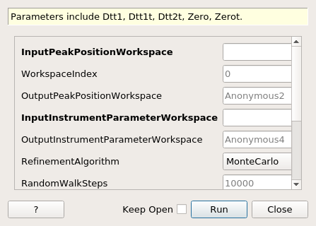
RefinePowderInstrumentParameters v3

Summary ¶

Parameters include Dtt1, Dtt1t, Dtt2t, Zero, Zerot.

Properties ¶

Name	Direction	Type	Default	Description
InputPeakPositionWorkspace	Input	Workspace2D	Mandatory	Data workspace containing workspace positions in TOF agains dSpacing.
WorkspaceIndex	Input	number	0	Workspace Index of the peak positions in PeakPositionWorkspace.
OutputPeakPositionWorkspace	Output	Workspace2D		Output data workspace containing refined workspace positions in TOF agains dSpacing.
InputInstrumentParameterWorkspace	Input	TableWorkspace	Mandatory	INput tableWorkspace containg instrument’s parameters.
OutputInstrumentParameterWorkspace	Output	TableWorkspace		Output tableworkspace containing instrument’s fitted parameters.
RefinementAlgorithm	Input	string	MonteCarlo	Algorithm to refine the instrument parameters. Allowed values: [‘OneStepFit’, ‘MonteCarlo’]
RandomWalkSteps	Input	number	10000	Number of Monte Carlo random walk steps.
MonteCarloRandomSeed	Input	number	0	Random seed for Monte Carlo simulation.
StandardError	Input	string	ConstantValue	Algorithm to calculate the standard error of peak positions. Allowed values: [‘ConstantValue’, ‘UseInputValue’]
Damping	Input	number	1	Damping factor for (1) minimizer ‘Damped Gauss-Newton’. (2) Monte Carlo.
AnnealingTemperature	Input	number	1	Starting annealing temperature.
MonteCarloIterations	Input	number	100	Number of iterations in Monte Carlo random walk.
ChiSquare	Output	number

Description ¶

This algorithm refines the instrumental geometry parameters for powder diffractomers. The parameters that can be refined are Dtt1, Zero, Dtt1t, Dtt2t, Zerot, Width and Tcross.

It serves as the second step to fit/refine instrumental parameters that will be introduced in Le Bail Fit. It uses the outcome from FitPowderDiffPeaks algorithm.

Introduction ¶

In order to do Rietveld refinement to experimental data, the diffractometer’s profile should be calibrated by the standards, such as LaB6 or Ni, with known crystal structure and lattice parameters.

For POWGEN and NOMAD, the type of the instrument profile is back-to-back exponential function convoluted with pseudo voigt of thermal neutron and epithermal neutron. It means that each diffraction peak is a back-to-back exponential,

\[I\frac{AB}{2(A+B)}\left[ \exp \left( \frac{A[AS^2+2(x-X0)]}{2}\right) \mbox{erfc}\left( \frac{AS^2+(x-X0)}{S\sqrt{2}} \right) + \exp \left( \frac{B[BS^2-2(x-X0)]}{2} \right) \mbox{erfc} \left( \frac{[BS^2-(x-X0)]}{S\sqrt{2}} \right) \right].\]

with peak parameter \(A\), \(B\), \(X_0\) and \(S\)

And their corresponding peak parameters are functions described as:

\[ \begin{align}\begin{aligned}n_{cross} = \frac{1}{2} \text{erfc}(Width(xcross\cdot d^{-1}))\\TOF_e = Zero + Dtt1\cdot d\\TOF_t = Zerot + Dtt1t\cdot d - Dtt2t \cdot d^{-1}\end{aligned}\end{align} \]

Final Time-of-flight is calculated as:

\[TOF = n_{cross} TOF_e + (1-n_{cross}) TOF_t\]

Formula for calculating \(A(d)\), \(B(d)\), \(\sigma(d)\) and \(\gamma(d)\)¶

\(\alpha(d)\):

\[ \begin{align}\begin{aligned}\alpha^e(d) = \alpha_0^e + \alpha_1^e d_h\\\alpha^t(d) = \alpha_0^t - \frac{\alpha_1^t}{d_h}\\\alpha(d) = \frac{1}{n\alpha^e + (1-n)\alpha^t}\end{aligned}\end{align} \]

\(\beta(d)\):

\[ \begin{align}\begin{aligned}\beta^e(d) = \beta_0^e + \beta_1^e d_h\\\beta^t(d) = \beta_0^t - \frac{\beta_1^t}{d_h}\\\beta(d) = \frac{1}{n\alpha^e + (1-n)\beta^t}\end{aligned}\end{align} \]

For \(\sigma_G\) and \(\gamma_L\), which represent the standard deviation for pseudo-voigt

\[ \begin{align}\begin{aligned}\sigma_G^2(d_h) = \sigma_0^2 + (\sigma_1^2 + DST2(1-\zeta)^2)d_h^2 + (\sigma_2^2 + Gsize)d_h^4\\\gamma_L(d_h) = \gamma_0 + (\gamma_1 + \zeta\sqrt{8\ln2DST2})d_h + (\gamma_2+F(SZ))d_h^2\end{aligned}\end{align} \]

The analysis formula for the convoluted peak at \(d_h\)

\[\Omega(TOF(d_h)) = (1-\eta(d_h))N\{e^u\text{erfc}(y)+e^v\text{erfc}(z)\} - \frac{2N\eta}{\pi}\{\Im[e^pE_1(p)]+\Im[e^qE_1(q)]\}\]

where

\[ \begin{align}\begin{aligned}\text{erfc}(x) = 1-\text{erf}(x) = 1-\frac{2}{\sqrt{\pi}}\int_0^xe^{-u^2}du\\E_1(z) = \int_z^{\infty}\frac{e^{-t}}{t}dt\\u = \frac{1}{2}\alpha(d_h)(\alpha(d_h)\sigma^2(d_h)+2x)\\y = \frac{\alpha(d_h)\sigma^2(d_h)+x}{\sqrt{2\sigma^2(d_h)}}\\p = \alpha(d_h)x + \frac{i\alpha(d_h)H(d_h)}{2}\\v = \frac{1}{2}\beta(d_h)(\beta(d_h)\sigma^2(d_h)-2x)\\z = \frac{\beta(d_h)\sigma^2(d_h)-x}{\sqrt{2\sigma^2(d_h)}}\\q = -\beta(d_h)x + \frac{i\beta(d_h)H(d_h)}{2}\end{aligned}\end{align} \]

\(\text{erfc}(x)\) and \(E_1(z)\) will be calculated numerically.

Break down the problem ¶

If we can do the single peak fitting on each single diffraction peak in a certain range, then we can divide the optimization problem into 4 sub problems for \(X_0\), \(A\), \(B\) and \(S\), with the constraint on \(n\), the ratio between thermal and epi thermal neutrons.

The function to fit is

\(X_0\):

\[TOF\_h = n(Zero + Dtt1\cdot d) + (1-n)(Zerot + Dtt1t\cdot d + Dtt2t/d)\]

\(A\):

\[\alpha(d) = \frac{1}{n\alpha^e + (1-n)\alpha^t}\]

\(B\):

\[\beta(d) = \frac{1}{n\alpha^e + (1-n)\beta^t}\]

\(S\):

\[\sigma_G^2(d_h) = \sigma_0^2 + (\sigma_1^2 + DST2(1-\zeta)^2)d_h^2 + (\sigma_2^2 + Gsize)d_h^4\]

with constraint:

\[n = 1/2 \text{erfc}(W\cdot (1-Tcross/d))\]

The coefficients in this function are strongly correlated to each other.

RefinePowderInstrumentParameters v3¶

Summary ¶

See Also ¶

Properties ¶

Description ¶

Introduction ¶

Formula for calculating \(A(d)\), \(B(d)\), \(\sigma(d)\) and \(\gamma(d)\)¶

Break down the problem ¶

Current Implementation ¶

Refinement Algorithm ¶

DirectFit ¶

MonteCarlo ¶

Constraint ¶

How to use algorithm with other algorithms ¶

Usage ¶

Source ¶