\(\renewcommand\AA{\unicode{x212B}}\)
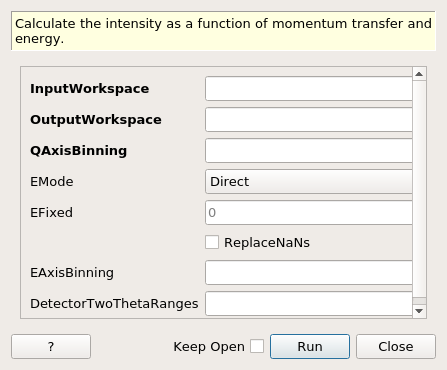
SofQWNormalisedPolygon dialog.
Table of Contents
| Name | Direction | Type | Default | Description |
|---|---|---|---|---|
| InputWorkspace | Input | MatrixWorkspace | Mandatory | Reduced data in units of energy transfer DeltaE. The workspace must contain histogram data and have common bins across all spectra. |
| OutputWorkspace | Output | MatrixWorkspace | Mandatory | The name to use for the q-omega workspace. |
| QAxisBinning | Input | dbl list | Mandatory | The bin parameters to use for the q axis (in the format used by the Rebin v1 algorithm). |
| EMode | Input | string | Mandatory | The energy transfer analysis mode (Direct/Indirect). Allowed values: [‘Direct’, ‘Indirect’] |
| EFixed | Input | number | 0 | The value of fixed energy: \(E_i\) (EMode=Direct) or \(E_f\) (EMode=Indirect) (meV). Must be set here if not available in the instrument definition. |
| ReplaceNaNs | Input | boolean | False | If true, all NaN values in the output workspace are replaced using the ReplaceSpecialValues algorithm. |
| EAxisBinning | Input | dbl list | The bin parameters to use for the E axis (optional, in the format used by the Rebin v1 algorithm). | |
| DetectorTwoThetaRanges | Input | TableWorkspace | A table workspace use by SofQWNormalisedPolygon containing a ‘Detector ID’ column as well as ‘Min two theta’ and ‘Max two theta’ columns listing the detector’s min and max scattering angles in radians. |
Converts a 2D workspace from units of spectrum number/energy transfer to the intensity as a function of momentum transfer \(Q\) and energy transfer \(\Delta E\).
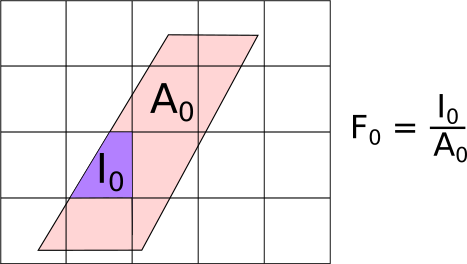
As shown in the figure, the input grid (pink-shaded parallelopiped, aligned in scattering angle and energy transfer) is not parallel to the output grid (square grid, aligned in \(Q\) and energy). This means that the output bins will only ever partially overlap the input data. To account for this, the signal \(Y\) and errors \(E\) in the new bins are calculated as:
In addition to weighting the signal and error values, the total fractional weights:
are also stored in the output of this algorithm which is a new workspace type: RebinnedOutput. To see why this is needed, consider rebinning the output on a larger grid:
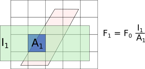
If the fractional weights are not chained as shown, then the area shaded in a lighter blue under \(A_1\) (where originally there was no data) would be included in the weights, which would be an overestimate of the actual weights, leading to an overestimate of the signal and error.
Finally, if there is a bin in the output grid which only has a very small overlap with the input grid (for example at the edges of the detector coverage), the fractional weight \(F\) of this bin, and hence its signal \(Y\) and error \(E\) would be very small compared to its neighbours. Thus, for display purposes, the actual signal and errors stored in a RebinnedOutput are renomalised by the weights:
at the end of the algorithm. The biggest consequence of this method is that in places where there are no counts (\(Y=0\)) and no acceptance (no fractional areas, \(F=0\)), \(Y/F=\)nan-s will result.
The algorithm operates in non-PSD mode by default. This means that the
scattering angle \(2\theta\) range covered by a detector is calculated for
each detector individually. For grouped detectors, it is the minimum and
maximum \(2\theta\) of all detectors in the group. The computation is
accurate for simple detector shapes (cylinder, cuboid); for other shapes a
more rough method is used. It is possible to provide precalculated
per-detector \(2\theta\) values using the DetectorTwoThetaRanges input
property.
PSD mode will determine the detector \(2\theta\) ranges from the instrument geometry. This mode is activated by placing the following named parameter in the instrument definition file: detector-neighbour-offset. The integer value of this parameter should be the number of pixels that separates two pixels at the same vertical position in adjacent tubes.
See SofQWCentre v1 for centre-point binning or SofQWPolygon v1 for simpler and less precise but faster binning strategies. The speed-up is from ignoring the azimuthal positions of the detectors (as for the non-PSD mode in this algorithm) but in addition, SofQWPolygon v1 treats all detectors as being the same, and characterised by a single width in scattering angle. Thereafter, it weights the signal and error by the fractional overlap, similarly to that shown in the first figure above, but then discards the summed weights, producing a Workspace2D rather than a RebinnedOutput workspace.
Example - simple transformation of inelastic workspace:
# create sample inelastic workspace for MARI instrument containing 1 at all spectra
ws=CreateSimulationWorkspace(Instrument='MAR',BinParams='-10,1,10')
# convert workspace into Matrix workspace with Q-dE coordinates
ws=SofQWNormalisedPolygon(InputWorkspace=ws,QAxisBinning='-3,0.1,3',Emode='Direct',EFixed=12)

print("The converted X-Y values are:")
Xrow=ws.readX(59);
Yrow=ws.readY(59);
line1= " ".join('! {0:>6.2f} {1:>6.2f} '.format(Xrow[i],Yrow[i]) for i in range(0,10))
print(line1 + " !")
line2= " ".join('! {0:>6.2f} {1:>6.2f} '.format(Xrow[i],Yrow[i]) for i in range(10,20))
print(line2 + " !")
print('! {0:>6.2f} ------- !'.format(Xrow[20]))
Output:
The converted X-Y values are:
! -10.00   1.00  !  -9.00   1.00  !  -8.00   1.00  !  -7.00   1.00  !  -6.00   1.00  !  -5.00   1.00  !  -4.00   1.00  !  -3.00   1.00  !  -2.00   1.00  !  -1.00   1.00  !
!   0.00   1.00  !   1.00   1.00  !   2.00   1.00  !   3.00   1.00  !   4.00   1.00  !   5.00   1.00  !   6.00   1.00  !   7.00   1.00  !   8.00   1.00  !   9.00   1.00  !
!  10.00 ------- !
Categories: AlgorithmIndex | Inelastic\SofQW