\(\renewcommand\AA{\unicode{x212B}}\)
Other Plot Docs
3D Mesh Plots - Table of contents
Mesh Plots can only be accessed with a script, not through the Workbench interface Here the mesh is plotted as a Poly3DCollection Polygon.
These sample shapes can be created with SetSample v1, LoadSampleShape v1 or LoadSampleEnvironment v1 and copied using CopySample v1.
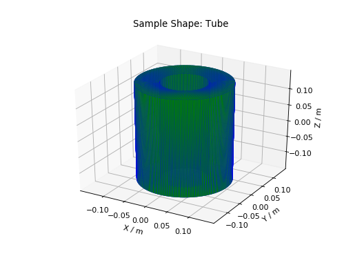
Plot a MeshObject from an .stl (or .3mf) file:
from mantid.simpleapi import *
import matplotlib.pyplot as plt
import numpy as np

from mpl_toolkits.mplot3d.art3d import Poly3DCollection
from mantid.api import AnalysisDataService as ADS

# load sample shape mesh file for a workspace
ws = CreateSampleWorkspace()
# alternatively: ws = Load('filepath') or ws = ADS.retrieve('ws')
ws = LoadSampleShape(ws, "tube.stl")

# get shape and mesh vertices
sample = ws.sample()
shape = sample.getShape()
mesh = shape.getMesh()

# Create 3D Polygon and set facecolor
mesh_polygon = Poly3DCollection(mesh, facecolors = ['g'], edgecolors = ['b'], alpha = 0.5, linewidths=0.1)

fig, axes = plt.subplots(subplot_kw={'projection':'mantid3d'})
axes.add_collection3d(mesh_polygon)

axes.set_mesh_axes_equal(mesh)
axes.set_title('Sample Shape: Tube')
axes.set_xlabel('X / m')
axes.set_ylabel('Y / m')
axes.set_zlabel('Z / m')

plt.show()
(Source code, png, hires.png, pdf)
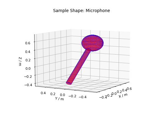
For help defining CSG Shapes and Rotations, see How To Define Geometric Shape. Plot a CSGObject defined in an XML string:
# import mantid algorithms, numpy and matplotlib
from mantid.simpleapi import *
import matplotlib.pyplot as plt
import numpy as np
from mpl_toolkits.mplot3d.art3d import Poly3DCollection

ws = CreateSampleWorkspace()

merge_xml = ' \
<cylinder id="stick"> \
<centre-of-bottom-base x="-0.5" y="0.0" z="0.0" /> \
<axis x="1.0" y="0.0" z="0.0" />  \
<radius val="0.05" /> \
<height val="1.0" /> \
</cylinder> \
\
<sphere id="some-sphere"> \
<centre x="0.7"  y="0.0" z="0.0" /> \
<radius val="0.2" /> \
</sphere> \
\
<rotate-all x="90" y="-45" z="0" /> \
<algebra val="some-sphere (: stick)" /> \
'

SetSample(ws, Geometry={'Shape': 'CSG', 'Value': merge_xml})

sample = ws.sample()
shape = sample.getShape()
mesh = shape.getMesh()

mesh_polygon = Poly3DCollection(mesh, edgecolors = 'blue', linewidths=0.1)
mesh_polygon.set_facecolor((1,0,0,0.5))

fig, axes = plt.subplots(subplot_kw={'projection':'mantid3d'})
axes.add_collection3d(mesh_polygon)

axes.set_mesh_axes_equal(mesh)
axes.view_init(elev=10, azim=-150)

axes.set_title('Sample Shape: Microphone')
axes.set_xlabel('X / m')
axes.set_ylabel('Y / m')
axes.set_zlabel('Z / m')

plt.show()
(Source code, png, hires.png, pdf)

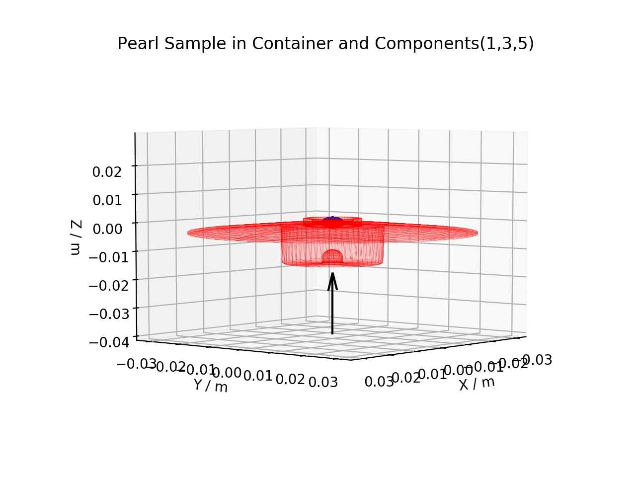
For help defining Containers and Components, see Sample Environment. Note Component index 0 is usually the Container.
ws = CreateSampleWorkspace()
LoadInstrument(Workspace=ws,RewriteSpectraMap=True,InstrumentName="Pearl")
SetSample(ws, Environment={'Name': 'Pearl'})

sample = ws.sample()
environment = sample.getEnvironment()

'''getMesh() to plot the Sample Shape'''
mesh = sample.getShape().getMesh()

'''getMesh() to plot the Container Shape'''
container_mesh = environment.getContainer().getShape().getMesh()

'''getMesh() to plot any Component Shape'''
# Component index 0 is the Container:
# container_mesh = environment.getComponent(0).getShape().getMesh()
component_mesh = environment.getComponent(2).getMesh()

# plot as meshes as previously described
(Source code, png, hires.png, pdf)
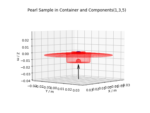
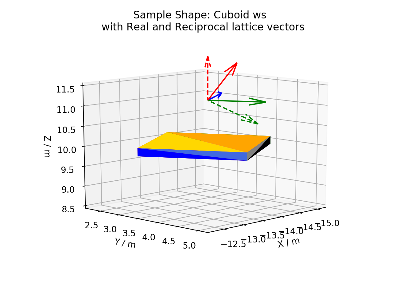
In the above Containers example, a black arrow for the beam direction was added. Below, the real and reciprocal lattice
vectors have been plotted (in solid and dashed linestyles respectively). Both of them make use of the arrow() function here:
def arrow(ax, vector, origin = None, factor = None, color = 'black',linestyle = '-'):
 if origin == None:
     origin = (ax.get_xlim3d()[1],ax.get_ylim3d()[1],ax.get_zlim3d()[1])
 if factor == None:
     lims = ax.get_xlim3d()
     factor = (lims[1]-lims[0]) / 3.0
 vector_norm = vector / np.linalg.norm(vector)
 ax.quiver(
      origin[0], origin[1], origin[2],
      vector_norm[0]*factor, vector_norm[1]*factor, vector_norm[2]*factor,
      color = color,
      linestyle = linestyle
 )

 # Create ws and plot sample shape as previously described

'''Add arrow along beam direction'''
source = ws.getInstrument().getSource().getPos()
sample = ws.getInstrument().getSample().getPos() - source
arrow(axes, sample, origin=(0,0,-0.04))

'''Calculate Lattice Vectors'''
SetUB(ws, a=1, b=1, c=2, alpha=90, beta=90, gamma=60)
if not sample.hasOrientedLattice():
   raise Exception("There is no valid lattice")
UB = np.array(ws.sample().getOrientedLattice().getUB())
hkl = np.array([[1.0,0.0,0.0],[0.0,1.0,0.0],[0.0,0.0,1.0]])
QSample = np.matmul(UB,hkl)
Goniometer = ws.getRun().getGoniometer().getR()
reciprocal_lattice = np.matmul(Goniometer,QSample)#QLab
real_lattice = (2.0*np.pi)*np.linalg.inv(np.transpose(reciprocal_lattice))

'''Add arrows for real and reciprocal lattice vectors'''
colors = ['r','g','b']
for i in range(3): # plot real_lattice with '-' solid linestyle
   arrow(axes, real_lattice[:,i], color = colors[i])
for i in range(3): # plot reciprocal_lattice with '--' dashed linestyle
   arrow(axes, reciprocal_lattice[:,i], color = colors[i], linestyle = '--')
(Source code, png, hires.png, pdf)

set_mesh_axes_equal()¶To centre the axes on the mesh and to set the aspect ratio equal, simply provide
the mesh of the largest object on your plot. If you want to add arrows to your plot,
you probably want to call set_mesh_axes_equal() first.
mesh = shape.getMesh()
mesh_polygon = Poly3DCollection(mesh, facecolors = facecolors, linewidths=0.1)
fig, axes = plt.subplots(subplot_kw={'projection':'mantid3d'})
axes.add_collection3d(mesh_polygon)

axes.set_mesh_axes_equal(mesh)
# then add arrows as desired
Other Plotting Documentation