\(\renewcommand\AA{\unicode{x212B}}\)

Asymmetric Pearson VII¶

Description¶

The asymmetric Pearson VII function (sometimes it is also referred to as the split-Pearson VII function) is a function that combines two Pearson VII distributions so to fit sharp peak curves [1]. It is useful for analysis of X-ray diffraction peaks which consist of two separable components.

In one of the representations, the asymmetric Pearson VII function \(A(x)\) can be written as a superposition of the “left” and “right” Pearson VII functions \(P_L(x)\) and \(P_R(x)\) [2],

\[A(x) = P_L(x) \, \theta(x_0 - x) + P_R(x) \, \theta(x - x_0) = P_L(x) \, \theta(x_0 - x) + P_R(x) \, \left(1 - \theta(x_0 - x) \right),\]

where \(x_0\) is the value when the function changes between the left and right Pearson VII, and this is usually chosen to be the peak centre. Moreover, \(\theta\) denotes the Heavyside step function with \(\theta(y \ge 0) = 1\) and \(\theta(y < 0)=0\), and \(P(x)\) denotes the Pearson VII function. This function takes four additional parameters and in general is defined as

\[P(x, h, x_0, \Gamma, m) = \frac{h}{\left(1 + \left[ \frac{2 (x-x_0) \sqrt{2^{1/m}-1}}{\Gamma} \right]^2 \right)^m} \, .\]

The four free parameters that the Pearson VII function \(P(x, h, x_0, \Gamma, m)\) takes represent the following quantities

\(h\) - the height of the peak
\(x_0\) - the location (centre) of the peak
\(\Gamma\) - the full width at half maximum
\(m\) - the function’s shape parameter

The parameter \(m\) can take values in the range \([0, \infty)\) and it determines whether \(P(x, h, x_0, \Gamma, m)\) is more close to a Lorentzian or a Gaussian. When \(m=1\) it’s a Lorentzian, whereas when \(m \rightarrow \infty\) it’s a Gaussian. The “left” and “right” Pearson VII functions \(P_L(x)\) and \(P_R(x)\) take identical parameters \(h, x_0, \Gamma\), but diffent \(m\), so that

\[P_L \equiv P(x, h, x_0, \Gamma, m_L),\]

\[P_R \equiv P(x, h, x_0, \Gamma, m_R).\]

In other words, it is assumed that the asymmetric Pearson VII function uses two halves of the Pearson VII with a common peak hight, peak centre, and full width at half maximum. As a result, the asymmetric Pearson VII distribution takes five parameters: \(h, x_0, \Gamma, m_L, m_R\). For the sake of stability of the numerical implementation of asymmetric Pearson VII distribution in Mantid, one operates with the weight parameter \(w \equiv 1/\Gamma\), i. e. \(A = A(x, h, x_0, w, m_L, m_R)\).

Analytic Derivatives¶

Below is the list of analytic derivatives of \(P = P(x, h, x_0, w, m)\) with respect to \(h, x_0, w, m\):

\[\frac{\partial P}{\partial h} = \frac{1}{d^m},\]

\[\frac{\partial P}{\partial x_0} = \frac{8 h m (x - x_0) \left( 2^{1/m} - 1 \right) w^2}{d^{m + 1}},\]

\[\frac{\partial P}{\partial w} = - \frac{8 h m (x - x_0)^2 \left( 2^{1/m} - 1 \right) w}{d^{m + 1}},\]

\[\frac{\partial P}{\partial m} = \frac{h}{d^{m + 1}} \left[ \frac{4 (x - x_0)^2 w^2 2^{1/m} \ln 2}{m d} - \ln \frac{1}{d} \right],\]

where

\[d \equiv \frac{1}{\left( 1 + 4 \left( x - x_0 \right)^2 \left( 2^{1/m} - 1 \right) w^2 \right)} \, .\]

Asymptotic Behavior¶

The numerical calculation of \(P(x, h, x_0, w, m)\) and its partial derivatives is complicated by singularities as \(m \rightarrow 0\). For this reason, one needs to operate with a limit of the corresponding expressions:

\[\lim_{m \rightarrow 0} P(x, h, x_0, w, m) = \frac{h}{2} \, ,\]

\[\lim_{m \rightarrow 0} \, \frac{\partial P(x, h, x_0, w, m)}{\partial h} = \frac{1}{2} \, ,\]

\[\lim_{m \rightarrow 0} \, \frac{\partial P(x, h, x_0, w, m)}{\partial x_0} = 0 \, ,\]

\[\lim_{m \rightarrow 0} \, \frac{\partial P(x, h, x_0, w, m)}{\partial w} = 0 \, ,\]

\[\lim_{m \rightarrow 0} \, \frac{\partial P(x, h, x_0, w, m)}{\partial m} = - \frac{h}{2} \, \ln \left[ 4(x-x_0)^2 w^2 \right] \, .\]

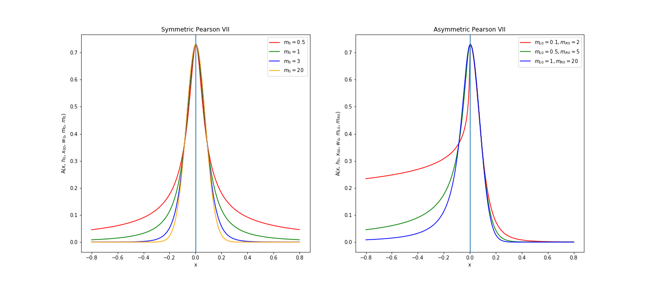
The figure below illustrates the comparison of shapes between various symmetric [3] and asymmetric Pearson VII distributions plotted for \(h_0 = 0.7297\), \(x_{00} = 0.0035\), \(w_0 = 5.7215\).

Properties (fitting parameters)¶

Name	Default	Description
PeakHeight	1.0	Hight of the peak
PeakCentre	0.0	Location of the peak
Width	0.1	Full width at half maximum
LeftShape	1.0	Left shape parameter
RightShape	1.0	Right shape parameter

References¶

[1]	Gupta, S. K. Peak Decomposition using Pearson Type VII Function, J. Appl. Cryst. (1998). 31, 474-476

[2]	Lifshin, E. (Ed.). (1999), X-ray Characterization of Materials, WILEY-VCH, https://doi.org/10.1002/9783527613748

[3]	http://pd.chem.ucl.ac.uk/pdnn/peaks/pvii.htm

Categories: FitFunctions | XrayDiffraction