\(\renewcommand\AA{\unicode{x212B}}\)

ClipPeaks v1

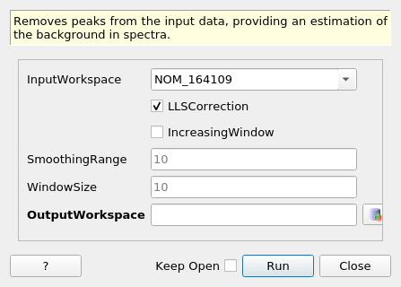
ClipPeaks dialog.

Summary

Removes peaks from the input data, providing an estimation of the background in spectra.

See Also

StripPeaks, StripVanadiumPeaks

Properties

Name	Direction	Type	Default	Description
InputWorkspace	Input	Workspace	Mandatory	The workspace containing the normalization data.
LLSCorrection	Input	boolean	True	Whether to apply a log-log-sqrt transformation to make data more sensitive to weaker peaks.
IncreasingWindow	Input	boolean	False	Use an increasing moving window when clipping.
SmoothingRange	Input	number	10	The size of the window used for smoothing data. No smoothing if set to 0.
WindowSize	Input	number	10	The size of the peak clipping window to be used.
OutputWorkspace	Output	Workspace	Mandatory	The workspace containing the normalization data.

Description

This algorithm is used to remove peaks from the input data, providing an estimation of the background in spectra. This is also known as a sensitive nonlinear iterative peak (SNIP) algorithm.

The input data can be optionally smoothed using a linear weighted average based on the value of the SmoothingRange parameter.

Smaller peaks present in the data can be exaggerated before clipping with the LLSCorrection option, which applies a log-log-sqrt function on the data. The inverse function is applied after the peaks are clipped.

Smoothing

If the smoothing window (s) is greater than 0, then the input is smoothed based on the following:

\[Y_{i}^{s} = \frac{ \sum_{r=-r_{max}}^{r_{max}} (r_{max} - \vert r \vert ) \cdot Y_{i+r} }{ \sum_{r=-r_{max}}^{r_{max}} (r_{max} - \vert r \vert ) }\]

where \(r_{max} = \frac{s}{2} + 1\). More information about smoothing can be found in [2].

Clipping

Peak clipping is done iteratively over the window size, \(w\). The order in which the data is clipped depends on whether an increasing or decreasing window is chosen: \(s = [1, 2, \cdots , w]\) or \(s = [w, w-1, \cdots , 1]\).

\[Y_{i}^{(k)} = \min \left( \frac{ \left[ Y_{i-s_k}^{(k-1)}, \cdots , Y_{i+s_k}^{(k-1)} \right] + \left[ Y_{i+s_k}^{(k-1)}, \cdots , Y_{i-s_k}^{(k-1)} \right] }{ 2 } \right )\]

where \((k)\) is the current iteration of \(Y_{i}\). If the LLS transformation is enabled, the inverse function is applied before doing the last operation:

\[Y_{i} = Y_{i}\ \cdot \ \left(\frac{ Y_{\min ( Y^{in} - Y )}^{in} }{ Y_{\min (Y^{in} - Y)} }\right)\]

Details about increasing vs decreasing windows can be found in [2] and an example C algorithm for the peak clipping algorithm described above can be seen in [1].

LLS Transformation

If the “LLSCorrection” option is true, then the input \(Y\) is transformed by the following before clipping is done:

\[Y^{\prime} = \log \left( \log \left( \sqrt{(Y + 1)} + 1 \right) + 1 \right)\]

After clipping, the inverse function is applied:

\[Y = ( \exp \, ( \exp( Y \, ) - 1 ) - 1)^2 - 1\]

More information about the LLS correction can be found in [1], [2], and [3].

Usage

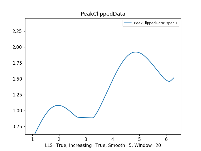
Example usage of using this algorithm on some data with random background noise and large peaks:

References

[1] (1,2)

Morháč, Miroslav, et al. Background Elimination Methods for Multidimensional Coincidence γ-Ray Spectra. Nuclear Instruments and Methods in Physics Research Section A: Accelerators, Spectrometers, Detectors and Associated Equipment 401.1 (1997): 113–132 doi: 10.1016/s0168-9002(97)01023-1

[2] (1,2,3)

Morháč, Miroslav, and Vladislav Matoušek. Peak Clipping Algorithms for Background Estimation in Spectroscopic Data. Applied Spectroscopy 62.1 (2008): 91–106 doi: 10.1366%2F000370208783412762

[3]

Morhac, Miroslav. Sophisticated algorithms of analysis of spectroscopic data. XII Advanced Computing and Analysis Techniques in Physics Research. 70 (2009): 77 doi: 10.22323/1.070.0077

Categories: AlgorithmIndex | Diffraction\Corrections

Source

Python: ClipPeaks.py