\(\renewcommand\AA{\unicode{x212B}}\)
LineProfile v1

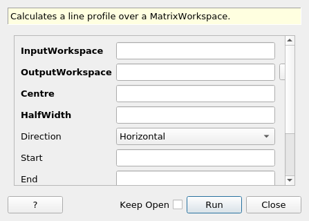
LineProfile dialog.
Summary
Calculates a line profile over a MatrixWorkspace.
See Also
Properties
Name |
Direction |
Type |
Default |
Description |
|---|---|---|---|---|
InputWorkspace |
Input |
Mandatory |
An input workspace. |
|
OutputWorkspace |
Output |
Mandatory |
A single histogram workspace containing the profile. |
|
Centre |
Input |
number |
Mandatory |
Centre of the line. |
HalfWidth |
Input |
number |
Mandatory |
Half of the width over which to calcualte the profile. |
Direction |
Input |
string |
Horizontal |
Orientation of the profile line. Allowed values: [‘Horizontal’, ‘Vertical’] |
Start |
Input |
number |
Optional |
Starting point of the line. |
End |
Input |
number |
Optional |
End point of the line. |
Mode |
Input |
string |
Average |
How the profile is calculated over the line width. Allowed values: [‘Average’, ‘Sum’] |
IgnoreInfs |
Input |
boolean |
False |
If true, ignore infinities when calculating the profile. |
IgnoreNans |
Input |
boolean |
True |
If true, ignore not-a-numbers when calculating the profile. |
Description
This algorithm extracts horizontal or vertical profiles from a MatrixWorkspace. The profile is returned as a single histogram workspace. Ragged workspaces are not supported.
The orientation of the profile is selected by the Direction property. By default, the line runs over the entire workspace. The length can be optionally limited by specifying the Start and/or the End properties. A region over which the profile is calculated is given by HalfWidth. The width is rounded to full bins so that partial bins are included entirely.
Special values can be completely ignored by the IgnoreNans and IgnoreInfs properties. If a segment of the line contains special values only, it will be set to NaN.
By default, the profile is calculated as an average over the line width. This behavior can be changed by the Mode property. The choices are:
- ‘Average’
Average the values. This is the default.
- ‘Sum’
Sum the values, weighting them by \(n / n_{tot}\) where \(n\) is the number of summed data points (excluding special values if IgnoreNans or IgnoreInfs is set) and \(n_{tot}\) is the total number of data points (including special values).
Profiles over distributions
Horizontal profiles over distribution data (Y divided by bin width) will be distributions as well.
However, vertical profiles over distribution data will be non-distributions, albeit the data is normalized by the profile width. To remove the normalization, it is possible to multiply the data by the total width of included bins. This information is contained in the vertical axis:
# line is a workspace created by LineProfile
axis = line.getAxis(1)
height = axis.getMax() - axis.getMin()
Ys = line.dataY(0)
Ys *= height
Es = line.dataE(0)
Es *= height
Usage
Example - Horizontal line profile
import numpy

ws = CreateSampleWorkspace(
    Function='Quasielastic Tunnelling',
    NumBanks=1
)

# Horizontal profile over spectra 5-10
horProfile = LineProfile(
    InputWorkspace=ws,
    Centre=7.5,
    HalfWidth=2.5,
    Start=3000,
    End=13000
)

indexMax = numpy.argmax(horProfile.readY(0))
epp = horProfile.readX(0)[indexMax]
print('Elastic peak at {}'.format(epp))
Output:
Elastic peak at 10000.0
Example - Vertical line profile
import numpy

ws = CreateSampleWorkspace(
    Function='Quasielastic Tunnelling',
    NumBanks=1
)

wsInTheta = ConvertSpectrumAxis(
    InputWorkspace=ws,
    Target='Theta'
)

# Verical cuts.

tofs = numpy.arange(3000, 7000, 500)
cutWSs = list()
for tof in tofs:
    cutWS = LineProfile(
        InputWorkspace=wsInTheta,
        OutputWorkspace='cut-at-{}-us'.format(tof),
        Direction='Vertical',
        Centre=float(tof),
        HalfWidth=250.0,
        Start=0.5,  # Degrees
        End=0.9
    )
    cutWSs.append(cutWS)

for cut in cutWSs:
    # Vertical axis holds the TOF bin edges of the cut
    axis = cut.getAxis(1)
    tofStart = axis.getValue(0)
    tofEnd = axis.getValue(1)
    # Notice the overlapping TOFs. This is because partial bins are
    # included in their entirety.
    print('Average intensity between {} and {} microsec: {:.03}'.format(
        tofStart, tofEnd, cut.readY(0)[0]))
Output:
Average intensity between 2600.0 and 3400.0 microsec: 0.1
Average intensity between 3200.0 and 3800.0 microsec: 0.1
Average intensity between 3600.0 and 4400.0 microsec: 0.164
Average intensity between 4200.0 and 4800.0 microsec: 0.1
Average intensity between 4600.0 and 5400.0 microsec: 0.1
Average intensity between 5200.0 and 5800.0 microsec: 0.1
Average intensity between 5600.0 and 6400.0 microsec: 0.227
Average intensity between 6200.0 and 6800.0 microsec: 0.1
Example - The ‘Sum’ mode
import numpy

ws = CreateSampleWorkspace(
    Function='Quasielastic Tunnelling',
    NumBanks=1
)

wsInTheta = ConvertSpectrumAxis(
    InputWorkspace=ws,
    Target='Theta'
)

# Lets assign NaNs to the lower left and upper right corners
# of the workspace.
for iVert in range(wsInTheta.getNumberHistograms()):
    for iHor in range(wsInTheta.blocksize()):
        if iVert + iHor < 60:
            ys = wsInTheta.dataY(iVert)
            ys[iHor] = numpy.nan
        elif iVert + iHor > 120:
            ys = wsInTheta.dataY(iVert)
            ys[iHor] = numpy.nan

centre = 0.6
width = 0.05
sumCutWS = LineProfile(wsInTheta, centre, width, Mode='Sum')

# When no NaNs are present both modes give the same result.
iElastic = sumCutWS.blocksize() // 2
y = sumCutWS.readY(0)[iElastic]
e = sumCutWS.readE(0)[iElastic]
print('Sum profile at elastic peak: {:.8f} +/- {:.10f}'.format(y, e))

# The weighting is apparent when the profile crosses some
# special values.
iEdge = sumCutWS.blocksize() // 6
y = sumCutWS.readY(0)[iEdge]
e = sumCutWS.readE(0)[iEdge]
print('Sum profile near NaNs: {:.11f} +/- {:.11f}'.format(y, e))
Sum profile at elastic peak: 103.45916358 +/- 10.1714877761
Sum profile near NaNs: 1.60000001019 +/- 2.52982213619
Categories: AlgorithmIndex | Utility
Source
C++ header: LineProfile.h
C++ source: LineProfile.cpp
