\(\renewcommand\AA{\unicode{x212B}}\)
NormaliseByDetector v1

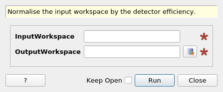
NormaliseByDetector dialog.
Summary
Normalise the input workspace by the detector efficiency.
See Also
Properties
Name |
Direction |
Type |
Default |
Description |
|---|---|---|---|---|
InputWorkspace |
Input |
Mandatory |
An input workspace in wavelength |
|
OutputWorkspace |
Output |
Mandatory |
An output workspace. |
Description
This algorithm is designed to normalise a workspace via detector efficiency functions. For this algorithm to work, the Instrument Definition File (IDF) must have fitting functions on the component tree. The setup information for this, as well as some examples, are provided below.
At a high-level, the algorithm does this:
Extract a detector efficiency function \(e = f(\lambda)\)
Using the bin boundaries on the input workspace, calculate efficiency Y and E values and generate a new workspace from the results
Divide the input workspace by the efficiency workspace
Prerequisites
The Input Workspace
The input workspace must be a MatrixWorkspace
The input workspace must have X-units of Wavelength, run ConvertUnits v1 on your input workspace if it is not already in Wavelength.
The input workspace must be a histogram workspace run ConvertToHistogram v1 on your input workspace if it is not already histogrammed.
The Instrument Definition File
Background
In brief, the components in the IDF file form a tree structure. Detectors and Instruments are both types of component. Detectors are ultimately children of Instruments in the tree structure. For a more complete description see IDF. The tree structure of the components, mean that fitting functions do not necessarily have to be assigned on a detector-by-detector basis. Applying a fit function to the instrument, will ensure that all subcomponents (including detectors), pick-up that function. However, functions assigned to lower-level components (such as detectors) take precedence over and existing functions that might exist on parent components (such as the instrument). You can even, have some parameters for a function provided against the detector, and pick up defaults from the bank, or instrument if they have been specified there.
Recommended Working
The IDF is intended to be a definitive description of the components in the instrument at any time. This should be the most generic form of the instrument setup possible. To complement this, you may provide additional Instrument Parameter files, which can be used to overload settings in the IDF for purposes of configuration and calibration. We strongly recommend that fitting functions are provided via Instrument Parameter Files rather than directly in the IDF. This will give you more flexibility to change your fitting functions without the problems of synchronising the IDF across Mantid, and possible corruption resulting from ad-hoc changes.
Instrument Parameter Files that take the form {InstrumentName}_Parameters.xml and live in the Instrument directory of Mantid are automatically loaded along with the IDF when a workspace is loaded into Mantid. However, you can apply any number of additional parameter files over the top of an existing workspace using LoadParameterFile v1.
Examples
Applying a LinearFunction to the whole instrument, hard-coded with A1=2 and A0=1. Fictional instrument is called basic_rect.
<parameter-file instrument = "basic_rect" date = "2012-01-31T00:00:00">
  <component-link name="basic_rect">
  <parameter name="LinearBackground:A0" type="fitting">
    <formula eq="1" result-unit="Wavelength"/>
    <fixed />
  </parameter>
  <parameter name="LinearBackground:A1" type="fitting">
    <formula eq="2" result-unit="Wavelength"/>
    <fixed />
  </parameter>
  </component-link>
</parameter-file>
Applying the same LinearFunction to two different detectors, with different coefficients is shown below:
<parameter-file instrument = "basic_rect" date = "2012-01-31T00:00:00">
<component-link name="bank1(0,0)">
   <parameter name="LinearBackground:A0" type="fitting">
       <formula eq="0" result-unit="Wavelength"/>
       <fixed />
   </parameter>
   <parameter name="LinearBackground:A1" type="fitting">
       <formula eq="1" result-unit="Wavelength"/>
       <fixed />
   </parameter>
</component-link>
<component-link name="bank2(0,0)">
   <parameter name="LinearBackground:A0" type="fitting">
       <formula eq="1" result-unit="Wavelength"/>
       <fixed />
   </parameter>
   <parameter name="LinearBackground:A1" type="fitting">
       <formula eq="1" result-unit="Wavelength"/>
       <fixed />
   </parameter>
</component-link>
</parameter-file>
In the following the LinearFunction A0 coefficient is set globally for all detectors at the instrument level, while the A1 coefficient is provided for each detector. In this way the Algorithm sees a complete definition for the Linear function (both A1 and A0) from two incomplete definitions on different components in the tree.
<parameter-file instrument = "basic_rect" date = "2012-01-31T00:00:00">
<component-link name="basic_rect">
<parameter name="LinearBackground:A0" type="fitting">
   <formula eq="3" result-unit="Wavelength"/>
   <fixed />
</parameter>
</component-link>
<component-link name="bank1(0,0)">
<parameter name="LinearBackground:A1" type="fitting">
   <formula eq="0" result-unit="Wavelength"/>
   <fixed />
</parameter>
</component-link>
<component-link name="bank2(0,0)">
<parameter name="LinearBackground:A1" type="fitting">
   <formula eq="1" result-unit="Wavelength"/>
   <fixed />
</parameter>
</component-link>
</parameter-file>
Usage
Example - A simple linear correction
import os

#create a param file
param_text = '''<parameter-file instrument = "basic_rect" date = "2012-01-31T00:00:00">
      <component-link name="basic_rect">
      <parameter name="LinearBackground:A0" type="fitting">
        <formula eq="1" result-unit="Wavelength"/>
        <fixed />
      </parameter>
      <parameter name="LinearBackground:A1" type="fitting">
        <formula eq="2" result-unit="Wavelength"/>
        <fixed />
      </parameter>
      </component-link>
    </parameter-file>'''

#find a suitable directory to save the param file
param_dir = config["defaultsave.directory"]
if not os.path.isdir(param_dir):
  #use the users home directory if default save is not set
  param_dir = os.path.expanduser('~')
param_file_path = os.path.join(param_dir,"NormByDet_Ex_param.xml")
#write the param file out
with open(param_file_path, "w") as param_file:
  param_file.write(param_text)


# a sample workspace with a sample instrument
ws = CreateSampleWorkspace()
# convert to Wavelength
ws = ConvertUnits(ws,"Wavelength")
#Load the param file into the workspace
LoadParameterFile(ws,param_file_path)

#Now we are ready to run the correction
wsCorrected = NormaliseByDetector(ws)

print("The correction will divide the data by an increasing linear function.")
print("f(x) = 2x + 1")
for i in range(0,wsCorrected.blocksize(),10):
  print("The correct value in bin {} is {:.2f} compared to {:.2f}".format(i,wsCorrected.readY(0)[i],ws.readY(0)[i]))

#clean up the file
if os.path.exists(param_file_path):
  os.remove(param_file_path)
Output:
The correction will divide the data by an increasing linear function.
f(x) = 2x + 1
The correct value in bin 0 is 0.28 compared to 0.30
The correct value in bin 10 is 0.14 compared to 0.30
The correct value in bin 20 is 0.09 compared to 0.30
The correct value in bin 30 is 0.07 compared to 0.30
The correct value in bin 40 is 0.06 compared to 0.30
The correct value in bin 50 is 1.63 compared to 10.30
The correct value in bin 60 is 0.04 compared to 0.30
The correct value in bin 70 is 0.04 compared to 0.30
The correct value in bin 80 is 0.03 compared to 0.30
The correct value in bin 90 is 0.03 compared to 0.30
Categories: AlgorithmIndex | CorrectionFunctions\NormalisationCorrections
Source
C++ header: NormaliseByDetector.h
C++ source: NormaliseByDetector.cpp
