\(\renewcommand\AA{\unicode{x212B}}\)
Elwin and I(Q, t)
Elwin
Provides an interface for the ElasticWindow algorithm, with the option of selecting the range to integrate over as well as the background range. An on-screen plot is also provided.
For workspaces that have a sample log, or have a sample log file available in the Mantid data search paths that contains the sample environment information the ELF workspace can also be normalised to the lowest temperature run in the range of input files.
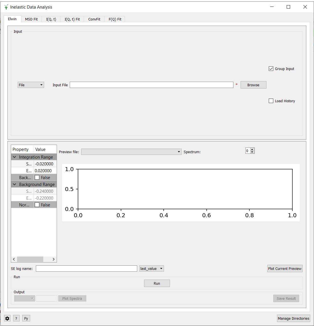
Elwin Options
- File or Workspace
Choose to load data from a file or a workspace by using this dropdown menu. See image below for demonstration of how to load files using either option.
- Input File
Specify a range of input files that are either reduced (_red.nxs) or \(S(Q, \omega)\).
- Group Input
The ElasticWindowMultiple algorithm is performed on the input files and returns a group workspace as the output. This option, if unchecked, will ungroup these output workspaces.
- Load History
If unchecked the input workspace will be loaded without it’s history.
- Integration Range
The energy range over which to integrate the values.
- Background Subtraction
If checked a background will be calculated and subtracted from the raw data.
- Background Range
The energy range over which a background is calculated which is subtracted from the raw data.
- Normalise to Lowest Temp
If checked the raw files will be normalised to the run with the lowest temperature, to do this there must be a valid sample environment entry in the sample logs for each of the input files.
- SE log name
The name of the sample environment log entry in the input files sample logs (defaults to ‘sample’).
- SE log value
The value to be taken from the “SE log name” data series (defaults to the specified value in the instrument parameters file, and in the absence of such specification, defaults to “last value”)
- Preview File
The workspace currently active in the preview plot.
- Spectrum
Changes the spectrum displayed in the preview plot.
- Plot Current Preview
Plots the currently selected preview plot in a separate external window
- Run
Runs the processing configured on the current tab.
- Plot Spectra
If enabled, it will plot the selected workspace indices in the selected output workspace.
- Save Result
Saves the result in the default save directory.
Elwin Example Workflow
The Elwin tab operates on _red and _sqw files. The files used in this workflow can
be produced using the run numbers 104371-104375 on the
Indirect Data Reduction interface in the ISIS Energy
Transfer tab. The instrument used to produce these files is OSIRIS, the analyser is graphite
and the reflection is 002.
Untick the Load History checkbox next to the file selector if you want to load your data without history.
Click Browse and select the files
osiris104371_graphite002_red,osiris104372_graphite002_red,osiris104373_graphite002_red,osiris104374_graphite002_redandosiris104375_graphite002_red. Load these files and they will be plotted in the mini-plot automatically.The workspace and spectrum displayed in the mini-plot can be changed using the combobox and spinbox seen directly above the mini-plot.
You may opt to change the x range of the mini-plot by changing the Integration Range, or by sliding the blue lines seen on the mini-plot using the cursor. For the purpose of this demonstration, use the default x range.
Tick Normalise to Lowest Temp. This option will produce an extra workspace with end suffix _elt. However, for this to work the input workspaces must have a temperature. See the description above for more information.
Click Plot Current Preview if you want a larger plot of the mini-plot.
Click Run and wait for the interface to finish processing. This should generate four workspaces ending in _eq, _eq2, _elf and _elt.
In the Output section, select the workspace ending with _eq and then choose some workspace indices (e.g. 0-2,4). Click Plot Spectra to plot the spectrum from the selected workspace.
Choose a default save directory and then click Save Result to save the output workspaces. The workspace ending in _eq will be used in the I(Q, t) Fit.
I(Q, t)
Given sample and resolution inputs, carries out a fit as per the theory detailed in the TransformToIqt algorithm.
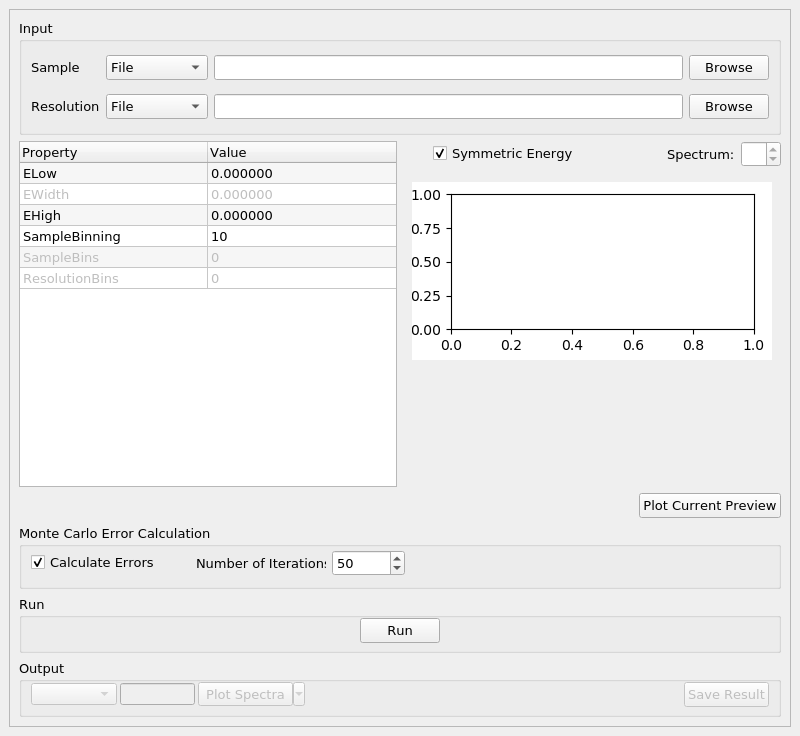
I(Q, t) Options
- Sample
Either a reduced file (_red.nxs) or workspace (_red) or an \(S(Q, \omega)\) file (_sqw.nxs) or workspace (_sqw).
- Resolution
Either a resolution file (_res.nxs) or workspace (_res) or an \(S(Q, \omega)\) file (_sqw.nxs) or workspace (_sqw).
- ELow, EHigh
The rebinning range.
- SampleBinning
The number of neighbouring bins are summed.
- Symmetric Energy Range
Untick to allow an asymmetric energy range.
- Spectrum
Changes the spectrum displayed in the preview plot.
- Plot Current Preview
Plots the currently selected preview plot in a separate external window
- Calculate Errors
The calculation of errors using a Monte Carlo implementation can be skipped by unchecking this option.
- Number Of Iterations
The number of iterations to perform in the Monte Carlo routine for error calculation in I(Q,t).
- Run
Runs the processing configured on the current tab.
- Plot Spectra
If enabled, it will plot the selected workspace indices in the selected output workspace.
- Plot Tiled
Generates a tiled plot containing the selected workspace indices. This option is accessed via the down arrow on the Plot Spectra button.
- Save Result
Saves the result workspace in the default save directory.
I(Q, t) Example Workflow
The I(Q, t) tab allows _red and _sqw for it’s sample file, and allows _red, _sqw and
_res for the resolution file. The sample file used in this workflow can be produced using the run
number 26176 on the Indirect Data Reduction interface in the ISIS
Energy Transfer tab. The resolution file is created in the ISIS Calibration tab using the run number
26173. The instrument used to produce these files is IRIS, the analyser is graphite
and the reflection is 002.
Click Browse for the sample and select the file
iris26176_graphite002_red. Then click Browse for the resolution and select the fileiris26173_graphite002_res.Change the SampleBinning variable to be 5. Changing this will calculate values for the EWidth, SampleBins and ResolutionBins variables automatically by using the TransformToIqt algorithm where the BinReductionFactor is given by the SampleBinning value. The SampleBinning value must be low enough for the ResolutionBins to be at least 5. A description of this option can be found in the A note on Binning section.
Untick Calculate Errors if you do not want to calculate the errors for the output workspace which ends with the suffix _iqt.
Click Run and wait for the interface to finish processing. This should generate a workspace ending with a suffix _iqt.
In the Output section, select some workspace indices (e.g.0-2,4,6) for a tiled plot and then click the down arrow on the Plot Spectra button before clicking Plot Tiled.
Choose a default save directory and then click Save Result to save the _iqt workspace. This workspace will be used in the I(Q, t) Fit Example Workflow.
A note on Binning
The bin width is determined from the energy range and the sample binning factor. The number of bins is automatically calculated based on the SampleBinning specified. The width is determined from the width of the range divided by the number of bins.
The following binning parameters cannot be modified by the user and are instead automatically calculated through the TransformToIqt algorithm once a valid resolution file has been loaded. The calculated binning parameters are displayed alongside the binning options:
- EWidth
The calculated bin width.
- SampleBins
The number of bins in the sample after rebinning.
- ResolutionBins
The number of bins in the resolution after rebinning. Typically this should be at least 5 and a warning will be shown if it is less.
Categories: Interfaces | Indirect