\(\renewcommand\AA{\unicode{x212B}}\)
LagrangeILLReduction v1

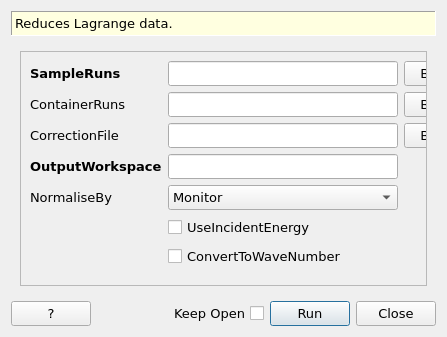
LagrangeILLReduction dialog.
Summary
Reduces Lagrange data.
Properties
Name |
Direction |
Type |
Default |
Description |
|---|---|---|---|---|
SampleRuns |
Input |
list of str lists |
Mandatory |
Sample run(s). |
ContainerRuns |
Input |
list of str lists |
Container run(s) (empty cell) |
|
CorrectionFile |
Input |
string |
Correction reference file. Allowed extensions: [‘.txt’] |
|
OutputWorkspace |
Output |
Mandatory |
The output workspace containing reduced data. |
|
NormaliseBy |
Input |
string |
Monitor |
What normalisation approach to use on data. Allowed values: [‘Monitor’, ‘None’] |
UseIncidentEnergy |
Input |
boolean |
False |
Show the energies as incident energies, not transfer ones. |
ConvertToWaveNumber |
Input |
boolean |
False |
Convert axis unit to energy in wave number (cm-1) |
Description
This algorithm reduces data from IN1 - Lagrange.
It can take as input multiple files from a single monochromator scan, the associated empty cell runs, and a correction file if needed. Reduction consists of multiplying the data by the correction factor from the correction file, and subtracting the empty cell from the raw data.
The X-axis of the result data can be offset by the incident energy using UseIncidentEnergy, and be converted to wave number instead of the default energy using ConvertToWaveNumber.
All the files in each field are merged together in a single curve, with very close points being removed to avoid interpolation artifacts.
Since the binning can be different between the raw data, the empty cell and the correction file, values are interpolated through numpy to provide matching values.
Note that for simplicity reasons, this algorithm is taking care of the loading and formatting of the ASCII data itself, and no separate loader exists for Lagrange data. Raw data can be checked by not filling any reduction parameter in this algorithm.
Usage
Simple Example with plotting of temperature vs initial energy
# full correction of a single monochromator scan, with multiple files
result = LagrangeILLReduction(SampleRuns='012869:012871',
                              ContainerRuns='012882:012884',
                              CorrectionFile='correction-water-cu220-2020.txt',
                              UseIncidentEnergy=False,
                              ConvertToWaveNumber=False)

run = result.getRun()
times = run.getLogData('time').value
eis = result.readX(0)
temperatures = run.getLogData('temperature').value

plt.plot(eis, temperatures)
plt.xlabel("Ei (meV)")
plt.ylabel("temperature (K)")
plt.show()
Multiple monochromators example
# complete reduction example for an entire experiment

# when reducing a scan spanning multiple monochromators, one needs to reduce each scan separately and then merge
# them together at the end

# import mantid algorithms
from mantid.simpleapi import *

# setting search directory for data
config.appendDataSearchDir("/path/to/data")

# setting data grouped by monochromator
samples = {"Cu220": 'raw_cu220_0, raw_cu220_1',
           "Si111": 'raw_si111_0',
           "Si311": 'raw_si311_0'}

# empty cell files
ec = {"Cu220": 'ec_cu220_0, ec_cu220_1',
      "Si111": 'ec_si111_0',
      "Si311": 'ec_si311_0'}

# correction files
corr = {"Cu220": "correction-factor-Cu220.txt",
        "Si111": "correction-factor-Si111.txt",
        "Si311": "correction_factor-Si311.txt"}

# treating data for each monochromator
for mono in samples.keys():
    LagrangeILLReduction(SampleRuns=samples[mono],
                         ContainerRuns=ec[mono],
                         CorrectionFile=corr[mono],
                         OutputWorkspace=mono,
                         UseIncidentEnergy=False,
                         ConvertToWaveNumber=False)

# stitching the results
Stitch(InputWorkspaces=",".join(samples.keys()), ReferenceWorkspace='Si311', OutputWorkspace="stitched")

# plotting all results
plotSpectrum(workspaces=list(samples.keys()) + ['stitched'], indices=0)
Categories: AlgorithmIndex | ILL\Indirect
Source
Python: LagrangeILLReduction.py
